Notes of Will Sawin first Hadamard lecture, 15-05-2023

Number theory over function fields

1. The classical theory

Let us start with classical stuff.

Theorem 1 (Dirichlet) ${N}$ a positive integer, ${a}$ an integer. There exist infinitely many prime numbers ${p}$ such that ${p=a \mod N}$ if and only if ${gcd(a,N)=1}$ .

A more precise statement is the prime number theorem on arithmetic progressions:

$\displaystyle \#\{p\in \mathcal{P}\,;\,p=a\mod N,\, p<x\}=\frac{1}{\phi(N)}\int_{2}^{x}\frac{dy}{\log y}+O_N (xe^{-C\sqrt{\log x}})$

for some explicit ${C}$ .

In other words, remainders mod ${N}$ of primes are evenly distributed.

The proofs of both theorems rely on properties of Dirichlet characters.

Definition 2 A function ${\chi:{\mathbb Z}^{>0}\rightarrow{\mathbb C}}$ is a Dirichlet character mod ${N}$ if

${\chi(mn)=\chi(m)\chi(n)}$ for all ${m,n}$ ,

${\chi(d+N)=\chi(d)}$ for all ${d}$ ,

${\chi(d)=0\iff gcd(d,N)\not=1}$ .

From a Dirichlet character, one constructs a Dirichlet ${L}$ -function

$\displaystyle L(x,\chi)=\sum_{n=1}^{\infty}\chi(n)n^{-s}=\prod_{p \in \mathcal{P}}\frac{1}{1-\chi(p)p^{-s}}.$

1.1. Properties

If ${\chi\not=\chi_0}$ , the trivial character, then ${L(s,\chi)}$ is entire. Dirichlet’s theorem follows from ${L(1,\chi)\not=0}$ . The prime number theorem on arithmetic progressions follows from ${L(1+t,\chi)\not=0}$ for all ${t\in{\mathbb R}}$ and on a neighborhood of that line. Improving the remainder to be polynomial of degree ${\alpha}$ is ${x}$ amounts to nonvanishing of ${L(s,\chi)}$ on ${\Re(s)>\alpha}$ . This is hard. The special case ${\alpha=\frac{1}{2}}$ is known as Generalized Riemann Hypothesis.

If one thinks of primes as random, i.e. an integer ${x}$ has a probability to be prime which is ${\frac{1}{\log x}}$ , the expected error from this random model is ${O_\epsilon((x/N)^{\frac{1}{2}+\epsilon})}$ .

Other interesting questions about Dirichlet ${L}$ -functions are statistical: what happens on the average over ${\chi}$ ?

1.2. Example: moments

We are interested in

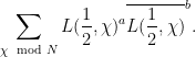
$\displaystyle \sum_{\chi\mod N}L(\frac{1}{2},\chi)^a\overline{L(\frac{1}{2},\chi)}^b.$

An exact expression is known only for ${a\le 2}$ , ${b\le 2}$ or ${a=3}$ , ${b=0}$ .

2. Function fields

These problems being too hard, I will study similar questions in a different, hopefully easier, setting. Let ${F_q}$ denote a field with ${q}$ elements, ${F_q[t]}$ denotes the ring of polynomials with coefficients in ${F_q}$ . I intend to replace integers with ${F_q[t]}$ . For instance, the Euclidean algorithm works on polynomials.

I denote by ${F_q[t]^+}$ the set of monic polynomials (thought of as an analogue of positive integers).

For ${f\in F_q[t]}$ , its absolute value is ${|f|=q^{\mathrm{deg(f)}}}$ , which is equal to the cardinality of the quotient ring ${F_q[t]/fF_q[t]}$ .

The advantage of the this shift of setting is that new connections with other fields of mathematics appear. Today, I will give one instance of that.

2.1. Dirichlet characters

Say that a function ${\chi:F_q[t]^+\rightarrow{\mathbb C}}$ is a Dirichlet character mod ${g\in F_q[t]^+}$ if

${\chi(fh)=\chi(f)\chi(h)}$ for all ${f,h\in F_q[t]^+}$ ,
${\chi(f+gh)=\chi(f)}$ for all ${f,g\in F_q[t]^+}$ ,
${\chi(f)=0\iff gcd(f,g)\not=1}$ .

The Dirichlet ${L}$ -function is

$\displaystyle L(s,\chi)=\sum_{f\in F_q[t]^+}\chi(f)|f|^{-s}.$

It is a power series in ${q^{-s}}$ . ${L(s,\chi)}$ is entire for ${\chi\not=\chi_0}$ , because it is a polynomial in ${q^{-s}}$ . Indeed,

$\displaystyle L(s,\chi)=\sum_{j=0}^{\infty}(\sum_{f\in F_q[t]^+,\,\mathrm{deg(f)=d}}\chi(f))q^{-ds}$

and the sum ${\displaystyle\sum_{f\in F_q[t]^+,\,\mathrm{deg(f)=d}}\chi(f)}$ vanishes for ${d\ge \mathrm{deg}(g)}$ , since each residue class mod ${g}$ occurs ${q^{d-\mathrm{deg}(g)}}$ times and, by orthogonality of characters, ${\sum_{a\in F_q[t]/g}\chi(a)=0}$ .

The Euler product formula holds,

$\displaystyle L(s,\chi)=\prod_{\pi\in F_q[t]^+,\,\pi\text{ irreducible}}\frac{1}{1-\chi(\pi)q^{-s\mathrm{deg}(\pi)}},$

showing that ${L(s,\chi)\not=0}$ for ${\Re(s)>1}$ . If we can improve nonvanishing we get information on the number of irreducible ${\pi\in F_q[t]^+}$ such that ${\pi=a\mod g}$ and ${\mathrm{deg}(\pi)=n}$ .

2.2. Generalized Riemann Hypothesis

In the new setting, the analogue of the Generalized Riemann Hypothesis is known, this is

Theorem 3 (Weil) ${L(s,\chi)\not=0}$ for ${\Re(s)>\frac{1}{2}}$ .

The proof is geometric.

Weil’s theorem implies that

$\displaystyle \#\{\pi\in F_q[t]^+\,\pi \text{ irreducible},\,\pi=a\mod g\,\mathrm{deg}(\pi)=n\}=\frac{q^n}{\phi(q)n}+O(\mathrm{deg}(g)q^{n/2}).$

2.3. Statistical issues

The theorem leaves open statistical questions about ${L(s,\chi)}$ . Katz, Katz-Sarnak, Deligne answered statistical questions in the limit where ${q}$ tends to infinity.

Definition 4 Say a character ${\chi}$ is primitive if there is no character ${\chi'}$ of smaller modulus ${g'}$ such that ${\chi(t)=\chi'(t)}$ for all ${f}$ with ${gcd(f,g)=1}$ .

Say ${\chi}$ is odd if ${\chi(g+\alpha)\not=1}$ for some ${\alpha\in F_q}$ .

Theorem 5 Assume ${\chi}$ is primitive and odd. Then ${L(s,\chi)}$ is a polynomial in ${q^{-s}}$ of degree exactly ${\mathrm{deg}(g)-1}$ with all roots on ${\frac{1}{2}+it\in{\mathbb C}}$ . It follows that ${L(s,\chi)}$ is the characteristic polynomial of ${q^{\frac{1}{2}-s}\theta_\chi}$ where ${\theta_\chi}$ is a unitary matrix.

Theorem 6 (Katz) If ${g}$ is squarefree and ${\mathrm{deg}(g)=m}$ , there a exists a map

$\displaystyle F:U(m-1)\rightarrow{\mathbb C}$

which is continuous, conjugacy invariant, such that

$\displaystyle \lim_{q\rightarrow\infty}\frac{1}{q^m}\sum_{\chi\text{ primitive, odd}}f(\theta_\chi)=\int_{U(m-1)}F(\theta)\,d\theta.$

In other words, the ${\theta_\chi}$ equidistribute in the unitary group as ${q}$ tends to infinity. It kills hope to control its nonvanishing simultaneously for all ${q}$ .

2.4. A sample result

Here is a theorem of mine.

Theorem 7 Let ${g}$ be squarefree of degree ${m}$ . Then

$\displaystyle \frac{q-1}{(q^m-1)(q-2)}\sum_{\chi\text{ primitive, odd}}L(s,\chi)^k = 1+O(k^m 2^{mk-k-m}q^{\frac{1-m}{2}}).$

In other words, the average over primitive, odd characters is 1 up to fluctuations which become small if ${q>k^2 2^{2(k-1)}}$ .

Whereas, in the classical setting, only a few moments are understood, in the new setting one can study arbitrarily high moments, provided ${q}$ is large enough.

The question has a geometric nature because it involves counting solutions to polynomial equations over ${F_q}$ . Since the middle of XXth century, one knows that such a counting can follow from the same topological techniques used to describe solutions over the complex numbers.

2.5. Scheme of proof

Let me give a scheme of the proof of Theorem 7. By the Euler product formula, the lefthand sum can be rewritten

$\displaystyle \sum_\chi\sum_{f_1,\ldots,f_k\in F_q[t]^+}\chi(f_1\cdots f_k)q^{s(\sum\mathrm{deg}(f_i))}.$

For a fixed ${h\in F_q[t]^+}$ ,

$\displaystyle \sum_{\chi\text{ odd}} \chi(h)=\begin{cases} 1 & \text{ if }h=1\mod g, \\ -\frac{1}{q-2} & \text{ if }h=\alpha\mod g,\,\alpha\in F_q[t]^\times, \\ 0 &\text{otherwise}. \end{cases}$

Therefore the sum becomes a sum over ${\alpha\in F_q[t]^\times}$ involving the number of ${f_1,\ldots,f_k\in F_q[t]^+}$ such that ${f_1\cdots f_k=\alpha\mod g}$ and ${\sum\mathrm{deg}(f_i)=n}$ .

This set is the union over ${k}$ -tuples of natural numbers summing to ${n}$ of sets, each of which is the set of solutions to ${m}$ equations in ${n}$ variables, over ${F_q}$ (the unknowns are the coefficients of the monic polynomials ${f_i}$ ).

The answer, obtained by Grothendieck’s school, can be found on the windows of Orsay’s math building.

Theorem 8 (Grothendieck-Lefschetz formula) Let ${X}$ be a scheme of finite type over ${F_q}$ . Then the number of points of ${X}$ over ${F_q}$ is

$\displaystyle \# X(F_q)=\sum_{j=0}^{2\mathrm{dim}(X)}(-1)^{i}\mathrm{trace}(Frob_q H^i(X(\overline{F_q}),{\mathbb Q}_\ell)).$

We also need

Theorem 9 (Deligne’s Riemann hypothesis) The eigenvalues of ${Frob_q}$ on ${H^i(X(\overline{F_q}),{\mathbb Q}_\ell)}$ are algebraic integers of absolue value ${\le q^{1/2}}$ .

This implies that the trace is bounded above by ${q^{1/2}}$ times the dimension of cohomology. This allows to conclude

Theorem 10 The number of solutions to the counting problem is

$\displaystyle \frac{1}{q^m-1}\sum_{j=0}^k (-1)^j\begin{pmatrix}k\\ j \end{pmatrix}\begin{pmatrix}n-jm+k-1\\ k-1 \end{pmatrix}q^{n-jk}+O(...).$

Thus we see that geometry has made it possible to go beyond the classical results in the function field setting.

Here is the key geometric statement. Let ${g}$ be a monic squarefree polynomial of degree ${m}$ over a field ${F}$ . Let ${a\in F[t]}$ be prime to ${g}$ . Consider the union of the schemes parametrizing the set of ${f_1,\ldots,f_k}$ whose product equals ${a\mod g}$ . Then the cohomology of the points over ${\bar F}$ splits as the sum of a boring piece (independent on ${a}$ ) and an interesting piece which is ${0}$ -dimensional if ${i\not=n-m,n+1-m}$ , and otherwise its dimension is at most

$\displaystyle \begin{cases} k^{m-1} \begin{pmatrix}mk-k-m+1\\ n-m+1 \end{pmatrix} & \text{ if }i=n+1-m, \\ (k^m-\begin{pmatrix}m+k-1\\ m-1 \end{pmatrix})\begin{pmatrix}mk-m-k\\ n-m \end{pmatrix} & \text{ if }i=n-m. \end{cases}$

	metric2011 on Notes of Sa’ar Hersonsky…
	CH on Videos
	Stefan Wenger on Notes of Stefan Wenger’s…
	Stefan Wenger on Notes of Stefan Wenger’s…
	Stefan Wenger on Notes of Stefan Wenger’s…

Notes of Will Sawin first Hadamard lecture, 15-05-2023

About metric2011

Leave a comment Cancel reply

Recent Posts

Recent Comments

Archives

Categories

Meta

Notes of Will Sawin first Hadamard lecture, 15-05-2023

Share this:

Related

About metric2011

Leave a comment Cancel reply

Recent Posts

Recent Comments

Archives

Categories

Meta