
When does 

The question goes back to Banach. This will be an excuse to review some modern tools. Banach space theory has evolved into metric geometry. The leitmotiv will be: how does one prove non-embeddability?
1. Linear embeddings
1.1. Banach’s question
Notation. 


Definition 1 A linear operator
between normed spaces is a
-isomorphic embedding, where
, if there exists
such that
,

Example 1
Remark. 
Question (Banach). For which 
Theorem 2 (Banach 1932, Paley 1936)
or
.
Theorem 3 (Kadec 1958)
Theorem 2 is much harder than Theorem 3 (although older).
1.2. Proof of Kadec’ theorem
Let 

Gaussians have the following property: if standard gaussian r.v. 


Define the embedding 

Then 


Question. Why doesn’t this work for other values of 

The answer arises in Paul Lévy’s book.
Theorem 4 (Levy 1951) Such random variables exist iff
. They are called standard
, they satisfy
Therefore,

is finite iff 
This shows that
Remark 1 To prove that
- If
is finitely representable in
and is separable, then
This ends our excursion in the construction of embeddings. From now on, we switch to nonembeddability results.
1.3. Linear distorsion
Definition 5 The linear distorsion of
is the smallest
and if
, by


Thus we have stated and partly proved that
Goal. Understand the asymptotics of 

Theorem 6 Let
. Then


Easy. The upper bounds are easy, the embedding is identity or identity to 
Our goal is to prove lower bounds, by designing invariants.
2. Smoothness and convexity in
2.1. Smoothness and convexity
Definition 7 (Ball – Carlen – Lieb 1993) Fix
. Say a Banach space
if
Fix
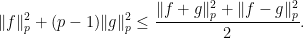
. Say a Banach space
-uniformly convex with constant
if


The best constants are denoted by 

Exercise. (Lindenstrauss’ duality formula à la Ball-Carlen-Lieb). For any normed space 

2.2. The case of
Theorem 8 (Clarkson’s inequality) For
.
For,
.
Proof. Since the inequality involves only 

By monotonicity of 

Theorem 9 For
,
.
For,
.
2.3. Two lemmata
The proof of Theorem 10 requires two lemmata, the first one is Bonami’s hypercontractivity inequality on the 
Lemma 10 (Bonami’s two-point inequality) Let
Proof. One can assume that 

The second lemma illustrates a general principle: an inequality for
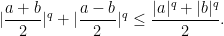
Lemma 11 (Hanner’s inequality) Let
,

One first checks that for ![{r\in[0,1]}](https://s0.wp.com/latex.php?latex=%7Br%5Cin%5B0%2C1%5D%7D&bg=ffffff&fg=000000&s=0&c=20201002)

satisfy
![\displaystyle \forall A,B\in{\mathbb R},\quad \max_{r\in[0,1]}\{\alpha(r)|A|^p+\beta(r)B^p\}\le |A+B|^p+|A-B|^p.](https://s0.wp.com/latex.php?latex=%5Cdisplaystyle++%5Cforall+A%2CB%5Cin%7B%5Cmathbb+R%7D%2C%5Cquad+%5Cmax_%7Br%5Cin%5B0%2C1%5D%7D%5C%7B%5Calpha%28r%29%7CA%7C%5Ep%2B%5Cbeta%28r%29B%5Ep%5C%7D%5Cle+%7CA%2BB%7C%5Ep%2B%7CA-B%7C%5Ep.+&bg=ffffff&fg=000000&s=0&c=20201002)
(again, one can assume that 

Hanner’s inequality follows: assuming that 


Integrating with respect to 


2.4. Proof of Theorem 10
Let 

Indeed, first apply Bonami’s inequality.
Conjecture. Does Hanner’s inequality hold in Schatten class, i.e. for matrices where the
Known for 


Conjecture. For
Theorem 12 (D. Schechtman 1995) Yes for
.
3. Martingales in Banach spaces
Definition 13 Let
such that for all
,

The basic example is

for given vectors 
Remark. If 


Definition 14 (Pisier 1975) A Banach space
,

These properties can be thought of as relaxations of the identity that holds in Hilbert space.
3.1. Smoothness/convexity versus type/cotype
These properties follow from the convexity properties introduced earlier.
Proposition 15 (Pisier)
Pisier’s renorming theorem states that the converse is true, up to changing for an equivalent norm.
The advantage of the type/cotype formulation is that the error is multiplicative, hence these properties are isomorphism invariant.
3.2. Proof of Pisier’s “smoothness implies type”
Let 


thus
Corollary 16 Let
.
If, then
If
, then


Beware that 


3.3. Proof of Theorem 7, type and cotype range
Let 


On the other hand,

This yields 
The proofs of the three other lower bounds on
Note that the argument used linearity very strongly.
4. Nonlinear embeddings
Given metric spaces 


Now we discretize spaces. Let ![{[m]_p^n=(\{1,2,\ldots,n\},\|.\|_p)}](https://s0.wp.com/latex.php?latex=%7B%5Bm%5D_p%5En%3D%28%5C%7B1%2C2%2C%5Cldots%2Cn%5C%7D%2C%5C%7C.%5C%7C_p%29%7D&bg=ffffff&fg=000000&s=0&c=20201002)

![{c_q([m]_p^n)}](https://s0.wp.com/latex.php?latex=%7Bc_q%28%5Bm%5D_p%5En%29%7D&bg=ffffff&fg=000000&s=0&c=20201002)
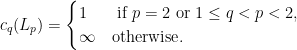
Theorem 17 Let
. Then


So we see that a phase transition occurs when 
In certain cases, the upper bounds are smart, but I will not focus on them.
In the unknown range 
![\displaystyle \min\{n^{1/q - 1/p},m^{1- q/p}\}\le_{p,q}c_q([m]_p^n)\le_{p,q}\min\{n^{1/q - 1/p},m^{1- 2/p}\}.](https://s0.wp.com/latex.php?latex=%5Cdisplaystyle++%5Cmin%5C%7Bn%5E%7B1%2Fq+-+1%2Fp%7D%2Cm%5E%7B1-+q%2Fp%7D%5C%7D%5Cle_%7Bp%2Cq%7Dc_q%28%5Bm%5D_p%5En%29%5Cle_%7Bp%2Cq%7D%5Cmin%5C%7Bn%5E%7B1%2Fq+-+1%2Fp%7D%2Cm%5E%7B1-+2%2Fp%7D%5C%7D.+&bg=ffffff&fg=000000&s=0&c=20201002)
The left-hand side would be sharp if the following was true: for every 


Theorem 18 (Bretagnolle – Dacunha-Castelle – Krivine 1965) This is true for
.
In my thesis, we have the following result:
Theorem 19 (Eskenazis – Naor 2016) For
, the space
does not embed in
5. Metric type
5.1. Enflo type
Definition 20 (Enflo 1969, modern terminology) A metric space
if for all
, for all
,

Remark. If 

and the righthand side is

so this is really a metric analogue of Rademacher type: for linear spaces,

Theorem 21 (Khot – Naor 2006) For normed linear spaces,

Proof. Let 

From martingale type, we know that 
where 
where 


which completes the proof.
The converse is a recent breakthrough, still in the linear case:
Theorem 22 (Ivanisvili – von Handel – Volberg 2020) For linear spaces, Rademacher type implies Enflo type.
5.2. Proof of distorsion lower bounds for 
The upper bound is easy (use global embedding of
Here is another easy lower bound:
![\displaystyle c_q([m]_p^n)\ge c_q([2]_p^n)=c_q(\{-1,1\}^n,\|.\|_p).](https://s0.wp.com/latex.php?latex=%5Cdisplaystyle++c_q%28%5Bm%5D_p%5En%29%5Cge+c_q%28%5B2%5D_p%5En%29%3Dc_q%28%5C%7B-1%2C1%5C%7D%5En%2C%5C%7C.%5C%7C_p%29.+&bg=ffffff&fg=000000&s=0&c=20201002)
Assume that 


(one sign change in 

6. Metric cotype
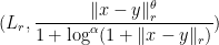
Formally, Rademacher cotype is the reverse of Rademacher type, but a naive delinearization does not work. The cube does not suffice, one needs an extra scaling factor 
Definition 23 (Mendel – Naor 2008) A metric space
with constant
if for any
such that any function
satisfies

Remark. As soon as 
Theorem 24 (Mendel – Naor 2008, Giladi – Mendel – Naor 2011) For normed spaces, Rademacher cotype is equivalent to metric cotype, and one can always take
.
The major open question is wether one can take 
Theorem 25 (Eskenazis – Mendel – Naor 2019) For normed spaces, martingale cotype implies metric cotype, with
.
6.1. Proof of the remaining distorsion lower bounds in Theorem 18
I will cheat and identify 
![{[m]_p^n}](https://s0.wp.com/latex.php?latex=%7B%5Bm%5D_p%5En%7D&bg=ffffff&fg=000000&s=0&c=20201002)
![\displaystyle [m]_p^n \subset {\mathbb Z}_{m}^{n}\subset [m+1]_p^{2n}.](https://s0.wp.com/latex.php?latex=%5Cdisplaystyle++%5Bm%5D_p%5En+%5Csubset+%7B%5Cmathbb+Z%7D_%7Bm%7D%5E%7Bn%7D%5Csubset+%5Bm%2B1%5D_p%5E%7B2n%7D.+&bg=ffffff&fg=000000&s=0&c=20201002)
We must show that
![\displaystyle c_q([m]_p^n)\ge_{p,q} m^{1-\frac{q}{p}} \quad \text{ if }m\le n^{1/q},](https://s0.wp.com/latex.php?latex=%5Cdisplaystyle++c_q%28%5Bm%5D_p%5En%29%5Cge_%7Bp%2Cq%7D+m%5E%7B1-%5Cfrac%7Bq%7D%7Bp%7D%7D+%5Cquad+%5Ctext%7B+if+%7Dm%5Cle+n%5E%7B1%2Fq%7D%2C+&bg=ffffff&fg=000000&s=0&c=20201002)
![\displaystyle c_q([m]_p^n)\ge_{p,q} n^{\frac{1}{q}-\frac{1}{p}} \quad \text{ if }m\ge n^{1/q}.](https://s0.wp.com/latex.php?latex=%5Cdisplaystyle++c_q%28%5Bm%5D_p%5En%29%5Cge_%7Bp%2Cq%7D+n%5E%7B%5Cfrac%7B1%7D%7Bq%7D-%5Cfrac%7B1%7D%7Bp%7D%7D+%5Cquad+%5Ctext%7B+if+%7Dm%5Cge+n%5E%7B1%2Fq%7D.+&bg=ffffff&fg=000000&s=0&c=20201002)
Since decreasing 


We see that we really need
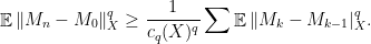
6.2. Proof of Theorem 26
The strategy is inspired from hypercontractivity: smoothing the space using an averaging operator puts functions closer to linear functions, i.e. leads us closer to the linear setting.
Given 

where 

If 


where (1) is an approximation term,
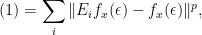
and (2) is a smoothing term,

We first estimate (1) with Hölder,

Jensen’s inequality gives

In other words,

which is ok since 
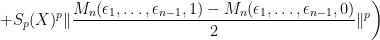
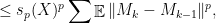
Next we bound (2). We can replace 


But

By martingale cotype,


Adding 
6.3. Final comment
What
