Notes of Corinna Ulcigrai’s Hadamard Lectures, june 2022

Parabolic dynamics

1. Survey

1.1. What does hyperbolic, elliptic mean in dynamics?

Let ${\phi_{\mathbb R}=(\phi_t)_{t\in{\mathbb R}}}$ be a dynamical system. Even if deterministic, it can exhibit a chaotic behaviour. This has several characteristics. One of them is the Butterfly effect: sensitive dependence on initial conditions (SDIC).

Definition 1 A flow ${\phi_{\mathbb R}}$ has SDIC if there exists ${K>0}$ such that ${\forall x\in X}$ , ${\forall \epsilon>0}$ , ${\exists y\in X}$ such that ${d(x,y)<\epsilon}$ and ${\exists t\in{\mathbb R}}$ such that ${d(\phi_t(x),\phi_t(y))\ge K}$ .

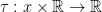
A quantitative measurement of SDIC is provided by the dependence of ${t}$ on ${\frac{1}{\epsilon}}$ .

Definition 2 Let ${S:{\mathbb R}_{>0}\rightarrow{\mathbb R}_{>0}}$ be a nondecreasing function. A flow ${\phi_{\mathbb R}}$ has SDIC of order ${S}$ if in the above definition, one can take ${t}$ such that ${S(t)\le \frac{1}{\epsilon}}$ .

This leads us to a rough division of dynamical systems:

Elliptic: no SDIC, or if any, subpolynomial.
Hyperbolic: SDIC is fast, exponential.
Parabolic: SDIC is slow, subexponential.

This trichotomy is advertised in Katok-Hasselblatt’s book.

For instance, entropy is a measure of chaos. Elliptic or parabolic dynamical systems have zero entropy. Hyperbolic dynamical systems have positive entropy.

1.2. Examples of elliptic dynamical systems

Circle diffeomorphisms.
Linear flows on the torus (these two examples are related, one is the suspension of the other).
Billiards in convex domains. Usually, there are many periodic orbits, trapping regions, caustics.

This the realm of Hamiltonian dynamics and KAM theory.

1.3. Examples of hyperbolic dynamical systems

Automorphisms of a torus which are Anosov, i.e. all eigenvalues have absolute values ${\not=1}$ . Then orbits diverge exponentially: if ${Av=\lambda v}$ , ${|\lambda|>1}$ , set ${y=x+\epsilon v}$ . Then ${T^n y=T^n x+\epsilon\lambda^n v}$ mod ${{\mathbb Z}^2}$ and ${|\epsilon\lambda^n|}$ reaches ${K=\frac{1}{2}}$ in time ${n}$ such that ${S(n)\le \frac{1}{\epsilon}}$ for ${S(t)=2|\lambda|^t}$ , an exponential.
Geodesic flows on constant curvature surfaces.
Sinai’s billiard: a rectangle with a circular obstacle. Somewhat equivalent to the motion of two hard spheres on a torus. Scattering occurs after hitting the obstacle, due to its strict convexity.

This is the realm of Anosov-Sinai and others’ dynamics. Structural stability occurs: hyperbolic systems form an open set.

1.4. Examples of parabolic dynamical systems

Horocycle flows on constant curvature surfaces. They were introduced by Hedlund, followed by Dani, Furstenberg, Marcus, Ratner.
Nilflows on nilmanifolds. If ${\Gamma<N}$ is a cocompact lattive in a nilpotent Lie group, let ${\phi_{\mathbb R}}$ be a ${1}$ -parameter subgroup of ${N}$ acting by right translations on ${N}$ . It descends to ${X=\Gamma\setminus N}$ . Both examples are algebraic, this provides us with tools to study them. They are a bit too special to illustrate parabolic dynamics.
Smooth area-preserving flows on higher genus surfaces.
Ehrenfest’s billiard: rectangular, with a rectangular obstacle. Here, SDIC is only caused by discontinuities due to corners. More generally, billiards in rational polygons (angles belong to ${\pi{\mathbb Q}}$ ), or equivalently linear flows on translation surfaces. This field is known as Teichmüller dynamics. Forni considers them as elliptic systems with singularities, I prefer to stress their parabolic character.

1.5. Uniformity

Within hyperbolic dynamics, there is a subdivision in uniformly hyperbolic, nonuniformly hyperbolic and partially hyperbolic.

In the same manner, we see horocycle flows as uniformly parabolic, and nilflows as partially parabolic, with both elliptic and parabolic directions. Area-preserving flows on surfaces have fixed points which introduce partially parabolic behaviour: shearing is uniform or not. However, there is no formal definition.

1.6. More examples of parabolic behaviours

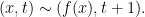
Parabolicity is not stable. However, Ravotti has discovered a ${1}$ -parameter perturbation of unipotent flows in ${\Gamma\setminus Sl(3,{\mathbb R})}$ .

A flow ${\tilde h_{\mathbb R}}$ is a time-change of a given flow ${h_{\mathbb R}}$ if there exists a function ${\tau:x\times{\mathbb R}\rightarrow{\mathbb R}}$ such that

$\displaystyle \forall x\in X,~\forall t\in{\mathbb R},\quad \tilde h_t(x)=h_{\tau(x,t)}(x).$

For ${\tilde h_{\mathbb R}}$ to be a flow, it is necessary that ${\tau}$ be a cocycle.

Both flows have the same trajectories. A feature of parabolic dynamics is that a typical time-change ${\tilde h_{\mathbb R}}$ is not isomorphic to ${h_{\mathbb R}}$ and has new chaotic features. Indeed, an isomorphism would solve the cohomology equation, and there are obstructions.

1.7. Program

Study smooth time-changes of algebraic flows.

Goes back to Marcus in the 1970’s. Algebraic tools break down, softer methods are required: geometric mechanisms. Also, we expect the features exhibited by time changes to be more typical.

2. Chaotic properties

2.1. Definitions

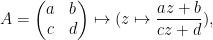
Definition 3 Let ${(X,\mathcal{A},\mu)}$ be a measure space with finite measure. Let ${\phi_{\mathbb R}}$ be a measure preserving flow. The trajectory of a point ${x\in X}$ is equidistributed with respect to ${\mu}$ if for every smooth observable ${f:X\rightarrow{\mathbb R}}$ ,

$\displaystyle \frac{1}{T}I_T(f,x):=\frac{1}{T}\int_{0}^{T}f(\phi_t(x))\,dt$ tends to ${0}$ as ${T}$ tends to ${\infty}$ .

${\phi_{\mathbb R}}$ is ergodic if ${\mu}$ almost every ${x\in X}$ has equidistributed orbit with respect to ${\mu}$ .

This is Boltzmann hypothesis.

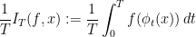
Definition 4 Say ${\phi_{\mathbb R}}$ is mixing if for all ${f,g\in L^2(X,\mu)}$ , the correlation

$\displaystyle \mathcal{C}_{f,g}(t):=\int f\circ\phi_t \,g\,d\mu-(\int f\,d\mu)(\int g\,d\mu)$ tends to ${0}$ as ${t}$ tends to ${\infty}$ .

This means decorrelation of functions. This implies ergodicity.

The speed at which decorrelation occurs is a significative feature too.

Definition 5 The speed of mixing is a function ${S:{\mathbb R}_+\rightarrow{\mathbb R}_+}$ such that for all smooth observables ${f,g:X\rightarrow{\mathbb R}}$ , the correlation decays at speed ${S}$ , i.e.

$\displaystyle \mathcal{C}_{f,g}(t)=O(S(t))$ as ${t}$ tends to ${\infty}$ .

2.2. Relation to the trichotomy

Elliptic systems often are not ergodic, but even when they are, they are not mixing.

Hyperbolic and parabolic systems can be mixing, but at different speeds:

hyperbolic ${\Rightarrow}$ exponential decay of correlations.
in parabolic systems, we expect that, if mixing occurs, the decay of correlations is slower: polynomial or subpolynomial.

A related concept is that of polynomial deviations of ergodic averages: if ${f}$ is smooth and has vanishing integral, ${\phi_{\mathbb R}}$ s ergodic and ${x}$ is an equidistribution point,

$\displaystyle |I_T(f,x)|=O(T^\alpha) \quad \text{for some}\quad 0<\alpha<1,$

and no faster. This phenomenon was first discovered on horocycle flows, then Teichmüller flows (Zorich, experimentally, Kontsevitch-Zorich for a proof).

2.3. Other features

Spectral properties. Let ${U_t}$ be the operator ${f\mapsto f\circ\phi_t}$ on ${L^2}$ . Then ${U_t}$ is unitary. What is its spectrum?

Disjointness of rescalings. Rescaling means linear time change ${\tilde h_t=h_{kt}}$ .

3. Results

Horocycle flow is mixing (Ratner). The spectrum is Lebesgue absolutely continuous.

Time changes of horocycle flows are mixing (Marcus, by shearing). This can be made quantitative (Forni-Ulcigrai).

Disjointness of rescalings fails for horocycle flows, but hold for nontrivial time changes (Kanigowski-Ulcigrai and Flaminio-Forni). The spectrum is Lebesgue absolutely continuous as well.

Nilflows themselves are not mixing, but typical time changes of nilflows are mixing (Avila-Forni-Ravotti-Ulcigrai).

We shall see geometric mechanisms at work:

Mixing via shearing.
Ratner property of shearing.
Renormizable parabolic flows.
Deviations of ergodic integrals.

4. Horocycle flows

Today’s goal is to explain the technique of mixing by shearing.

4.1. Algebraic viewpoint

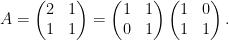
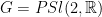
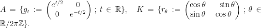
Consider ${G=PSl(2,{\mathbb R})}$ and its subgroups

$\displaystyle N=\{h_s:=\begin{pmatrix} 1 & s \\ 0 & 1 \end{pmatrix}\,,s\in{\mathbb R}\}, \quad N=\{h^-_s:=\begin{pmatrix} 1 & 0 \\ s & 1 \end{pmatrix}\,,s\in{\mathbb R}\},$

$\displaystyle A=\{g_t:=\begin{pmatrix} e^{t/2} & 0 \\ 0 & e^{-t/2} \end{pmatrix}\,;\,t\in{\mathbb R}\},\quad K=\{r_\theta :=\begin{pmatrix} \cos\theta & -\sin\theta \\ \sin\theta & \cos\theta \end{pmatrix}\,;\,\theta\in {\mathbb R}/2\pi{\mathbb Z}\}.$

Every matrix can be uniquely written ${g=h_s g_t r_\theta}$ , hence ${G=NAK}$ . The factors do not commute, because of the key relation

$\displaystyle g_t h_s = h_{e^{t}s} g_t.$

The key relation can be interpreted as a selfsimilarity property: ${h_\mathbb{R}}$ is a fixed point of renormalization by ${g_{\mathbb R}}$ .

Take a discrete and cocompact subgroup ${\Gamma<G}$ . Then ${A}$ and ${N}$ act on ${X=G/\Gamma}$ by left multiplication. The key relation implies that the rescaled flow $latex {h_{\mathbb R}^k=(h_{ks})_{s\in{\mathbb R}}}&fg=000000$ is conjugated to $latex {h_{\mathbb R}}&fg=000000$. This fails for other (nonrescaling) time changes, as I proved recently with Fraczek and Kanigowski.

4.2. Geometric viewpoint

Let ${\mathbb{H}}$ denote the upper half plane, with metric ${ds^2=\frac{dx^2+dy^2}{y^2}}$ .

Fact. ${G}$ acts isometrically and transitively on ${\mathbb{H}}$ , and this yields a diffeomorphism of ${G}$ with the unit tangent bundle ${T^1 \mathbb{H}}$ .

Indeed, the action is by Möbius transformations

$\displaystyle A=\begin{pmatrix} a & b \\ c & d \end{pmatrix}\mapsto (z\mapsto \frac{az+b}{cz+d}),$

on ${\mathbb{H}}$ , and by their derivatives on ${T^1 \mathbb{H}}$ .

With this identification, orbits of ${A}$ are curves which project to geodesics of ${\mathbb{H}}$ , and coincide with their lifts by their unit speed vector. On the other hand, orbits of ${N}$ are curves which projects to horocycles of ${\mathbb{H}}$ , and coincide with their lifts by their unit normal outward pointing vectors. Lifts by inward pointing normal vectors are orbits of ${N^-}$ .

${A=g_{\mathbb R}}$ is a hyperbolic flow: it contracts in the direction of ${N^-}$ -orbits, it dilates in the direction of ${N}$ -orbits,

4.3. Classical results

Let ${\mu}$ denote Haar measure on ${G}$ . It maps via ${G\rightarrow T^1\mathbb{H}\rightarrow\mathbb{H}}$ to hyperbolic volume. Consider the induced measure on ${X=G/\Gamma}$ (still denoted by ${\mu}$ ). Then ${\mu(X)<+\infty}$ and ${A}$ acts on ${X}$ by measure preserving transformations.

Then

${A}$ is ergodic (Hopf). It is far from being unique ergodic (plenty of periodic orbits).
${A}$ is mixing.
${N}$ is uniquely ergodic (Furstenberg). This means that every orbit is equidistributed with respect to ${\mu}$ .

5. Shearing

This is an alternate way to prove mixing. The idea goes back to Marcus (Annals of Math. 1977). Marcus covered a more general situation, and proved mixing of all orders (i.e. for multicorrelations, integrals involving an arbitrarily large number of functions).

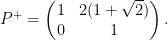
Let us shift viewpoint on the key relation. Let ${\gamma}$ be a piece of ${A}$ -orbit of length ${\sigma}$ . Let

$\displaystyle \gamma^s:=h_s\circ\gamma=\{h_s g_t x\,;\,0\le t \le \sigma\}.$

Then ${\gamma^s}$ is sheared or tilted in the direction of the geodesic flow.

Key idea in parabolic dynamics: In several parabolic systems, the Butterfly effect happens in a special way, e.g. shearing. Points nearby move parallel, but with different speeds. This implies that transverse arcs shear.

5.1. Recipe for mixing in parabolic dynamics

Here are the ingredients:

A uniquely ergodic flow ${\phi_{\mathbb R}}$ .
A transverse direction which is sheared in the direction of the flow.

By assumption, for every ${x\in X}$ , the trajectory ${\phi_{{\mathbb R}_+}(x)}$ equidistributes with respect to ${\mu}$ . We want to upgrade it to mixing, which is a property of sets: indeed

$\displaystyle \int f\circ\phi_t \,g\,d\mu \rightarrow (\int f\,d\mu)(\int g\,d\mu)$

is equivalent to

$\displaystyle \forall A,B\in\mathcal{A},\quad\mu(\phi_t(A)\cap B)\rightarrow \mu(A)\mu(B)$

i.e ${\phi_t(A)}$ equidistributes as ${t\rightarrow+\infty}$ .

The idea is to cover ${A}$ by short arcs in the transverse direction. We prove that each such arc equidistributes, and apply Fubini. I.e. if ${A=\bigcup \gamma_\alpha}$ , apply ${\phi_t}$ . Then ${\phi_t(A)=\bigcup\phi_t(\gamma_\alpha)}$ .

Each ${\phi_t(\gamma_\alpha)}$ becomes close to a long piece of orbit of ${\phi_{\mathbb R}}$ . By unique ergodicity, that piece equidistributes, and this implies equidistribution for ${\gamma_\alpha}$ .

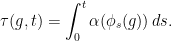
5.2. Time change

Let ${\tau:X\times{\mathbb R}\rightarrow {\mathbb R}}$ be a smooth time change, which is a cocycle with respect to a given smooth flow ${h_{\mathbb R}}$ , i.e.

$\displaystyle \tau(x,t+s)=\tau(x,t)+\tau(h_t(x),s).$

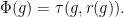
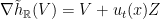
We are interested in the flow ${\tilde h}$ defined by

$\displaystyle h_t(x)=\tilde h_{\tau(x,t)}(x).$

The generator of ${\tau}$ is

$\displaystyle \alpha(x):=\frac{\partial \tau(x,t)}{\partial t}_{|t=0}.$

It is a smooth nonnegative function on ${X}$ . We assume that ${\int \alpha\,d\mu=1}$ . We denote ${\tilde h}$ by ${h^\alpha_{\mathbb R}}$ .

Remark. If ${h_{\mathbb R}}$ is generated by a smooth vectorfield ${U}$ , then ${\tilde h_{\mathbb R}}$ is generated by the vectorfield ${\frac{1}{\alpha}U}$ .

Theorem 6 (Forni-Ulcigrai) Let ${h_{\mathbb R}}$ be the horocyclic flow of a compact constant curvature surface. For any smooth function ${\alpha}$ , the flow ${h^\alpha_{\mathbb R}}$ is mixing, with quantitative estimates which imply that the spectrum is absolutely continuous with respect to Lebesgue measure.

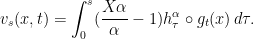
Lemma 7 Let ${X}$ denote the generator of ${g_{\mathbb R}}$ and ${U}$ the generator of ${h_{\mathbb R}}$ . Take a segment of ${g_{\mathbb R}}$ -orbit

$\displaystyle \gamma=\{g_t x\,;\,0\le t \le \sigma\}.$ Let $\displaystyle \gamma_s:=h^\alpha_s\circ\gamma.$ Then $\displaystyle \frac{d\gamma_s}{dt}=v_s(x,t)U_\alpha +X,$ where $\displaystyle v_s(x,t)=\int_{0}^{s}(\frac{X\alpha}{\alpha}-1)h^\alpha_\tau\circ g_t(x)\,d\tau.$

Remark. ${\int \frac{X\alpha}{\alpha}\,d\mu=0}$ , hence ${\int(\frac{X\alpha}{\alpha}-1)\,d\mu=-1}$ . Thus, as ${s}$ tends to ${+\infty}$ , ${\frac{1}{s}v_s(x,t)}$ tends to a finite limit, the shear rate.

Proof of Lemma. It relies on ${[U,X]=U}$ , which implies that ${[U_\alpha,X]=(\frac{X\alpha}{\alpha}-1)U_\alpha}$ .

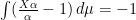
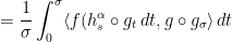
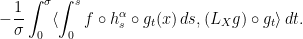
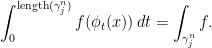
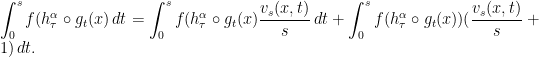
We see that we need compute integrals over sheared arcs ${\gamma_s}$ . Let ${f:X\rightarrow{\mathbb R}}$ be a smooth function. Then

$\displaystyle \int_{0}^{s}f(h^\alpha_\tau\circ g_t(x)\,dt =\int_{0}^{s}f(h^\alpha_\tau\circ g_t(x)\frac{v_s(x,t)}{s}\,dt+\int_{0}^{s}f(h^\alpha_\tau\circ g_t(x))(\frac{v_s(x,t)}{s}+1)\,dt.$

The second term is an ergodic integral which is easy to handle. The main term is the first term, which can be rewritten

$\displaystyle -\frac{1}{s}\int_{\gamma_s}f\hat U_\alpha,$

where ${i_{U_\alpha}\hat U_\alpha=1}$ , ${i_X \hat U_\alpha=0}$ .

To deduce mixing, one must estimate ${L^2}$ inner products ${\langle f\circ h^\alpha_s,a\rangle}$ . We integrate by parts

$\displaystyle \langle f\circ h^\alpha_s,g\rangle =\frac{1}{\sigma}\int_{0}^{\sigma}\langle f\circ h^\alpha_s\circ g_t,g\circ g_t\rangle\,dt$

$\displaystyle =\frac{1}{\sigma}\int_{0}^{\sigma}\langle f(h^\alpha_s\circ g_t\,dt,g\circ g_\sigma\rangle\,dt$

$\displaystyle -\frac{1}{\sigma}\int_{0}^{\sigma}\langle\int_{0}^{s}f\circ h^\alpha_s\circ g_t(x)\,ds,(L_Xg)\circ g_t\rangle\,dt.$

The second term is again an ergodic integral that tends to ${0}$ .

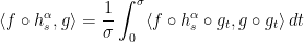
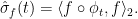
5.3. Quantitative equidistribution estimates

We are interested in ergodic integrals of the form

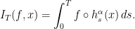
$\displaystyle I_T(f,x)=\int_{0}^{T}f\circ h^\alpha_s(x)\,ds.$

Flaminio-Forni treat the un-time-changed case ${\alpha=1}$ and show that

$\displaystyle \|I_T(f,x)\|_{L^\infty}\le C\, T^{(1+\nu_0)/2}$

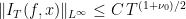
for some ${0<\nu_0\le 1}$ . One can adapt their arguments, using estimates by Bufetov-Forni, to the time-changed case, and get similar estimates.

5.4. Additional references

Marcus original technique already proved mixing. His setting was Anosov flows, with their stable and unstable foliations. From these, a flow ${h_{\mathbb R}}$ can be defined, which satisfies

$\displaystyle g_t \circ h_s =h_{ss^*(t,s,x)}\circ g_t,$

where $latex {s^*}&fg=000000$ has a continuous mixed partial second derivative $latex {\frac{\partial s^*}{\partial t \partial s}}&fg=000000$. So we see that time-changes were already in the picture.

Kushnirenko was able to prove mixing for smooth time-changes, assuming

$\displaystyle (KC)\quad\quad \|\frac{X\alpha}{\alpha}\|_{\infty}<1.$

Thus small time-changes are mixing. What about larger ones? This is still open.

Tiedra de Aldecoa uses a different method to prove absolute continuity of the spectrum for time changes satisfying (KC).

Generalizations. The setting is algebraic dynamics: a unipotent ${1}$ -parameter subgroup acting on ${G/\Gamma}$ , ${G}$ semisimple Lie group.

Lucia Simonelli (Forni’s student) could prove absolute continuity of the spectrum for time changes satisfying (KC).

Davide Ravotti (my student) could prove quantitative mixing.

Kanigowski and Ravotti could prove quantitative ${3}$ -mixing.

6. Heisenberg nilfows

Let ${H}$ denote the Lie group of unipotent ${3\times 3}$ matrices, with ${X,Y,Z}$ as standard generators of its Lie algebra, ${Z=[X,Y]}$ . Let ${\Gamma<H}$ be a discrete cocompact lattice (for instance, unipotent matrices with integer entries). We call ${X=\Gamma\setminus H}$ the Heisenberg nilmanifold. ${H}$ acts on ${X}$ by right multiplication. The action of a ${1}$ -parameter subgroup is called a nilflow.

6.1. Classical results

Auslander-Green-Hahn (1963) studied unique ergodicity of nilflows. They showed that is ${W\in Lie(H)}$ can be written ${W=aX+bY+cZ}$ , for the nilflow defined by ${W}$ ,

unique ergodicity ${\Leftrightarrow}$ ergodicity ${\Leftrightarrow}$ minimality ${\Leftrightarrow}$ ${a,b}$ and ${1}$ are rationally independent.

Rational independence means that no linear relation with nonzero integral coefficients ${ka+\ell b+ n=0}$ can hold.

In other words, if we project the situation to the ${2}$ -torus ${\bar X=\bar\Gamma\setminus\bar H}$ where ${\bar H=H/[H,H]}$ , ${\bar\Gamma=}$ , then the flow ${\phi^W_{\mathbb R}}$ projects to a flow ${\bar \phi_{\mathbb R}}$ on ${\bar X}$ , and

unique ergodicity for ${\phi_{\mathbb R}}$ ${\Leftrightarrow}$ unique ergodicity for ${\bar\phi_{\mathbb R}}$ .

Here, we have used a theorem of Furstenberg on skew-products of rotations of the circle.

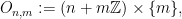
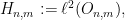
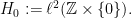
Definition 8 For real numbers ${\alpha,\beta\in{\mathbb R}}$ , let ${f_{\alpha,\beta}}$ be the diffeomorphism of the ${2}$ -torus defined by

$\displaystyle f_{\alpha,\beta}(x,y)=(x+\alpha,y+x+\beta) \mod {\mathbb Z}^2.$

In general, a skew-product over a map ${T:X\rightarrow X}$ is a map ${f:X\times Y\rightarrow X\times Y}$ which is fiber-preserving (with respect to the projection ${X\times Y\rightarrow X}$ ) and the permutation of fibers is given by ${T}$ . In the example at hand, ${f}$ is isometric on fibers.

6.2. First return map

Lemma 9 Assume that the Heisenberg nilflow ${\phi^W_{\mathbb R}}$ is uniquely ergodic. There is a transverse submanifold ${\Sigma\subset X}$ , diffeomorphic to a torus, such that the Poincaré return map ${P:\Sigma\rightarrow\Sigma}$ , given by ${P(g)=\Phi^W_{r(g)}(g)}$ , ${r}$ the first return time to ${\Sigma}$ , is one of the Furstenberg skew-products ${f_{\alpha,\beta}}$ .

Proof of the Lemma. ${\Sigma}$ lifts to a vertical plane ${{\exp(xX+zZ)\,;\,x,z\in {\mathbb R}}}$ in ${H}$ . Since ${X}$ and ${Z}$ commute, ${\Sigma}$ is diffeomorphic to a torus. If ${\phi^W_{\mathbb R}}$ is uniquely ergodic, ${b\not=0}$ , so ${\Sigma}$ is transverse to the flow.

We show that ${\frac{1}{b}}$ is a return time. We use the fact that ${\exp(-Y)\in\Gamma}$ . So using the Campbell-Hausdorff-Dynkin formula, we compute

$\displaystyle \exp(-Y)\exp(xX+zZ)\exp(\frac{W}{b}) =\exp((x+\frac{a}{b})X+(z+x+\frac{c}{b}+\frac{a}{2b})Z).$

This point belongs to ${\Sigma}$ , so ${P(x,z)=f_{\frac{a}{b},\frac{c}{b}+\frac{a}{2b}}(x,z)}$ .

6.3. Lack of mixing

The above Lemma shows th at we can now focus on Furstenberg skew-products. We shall see that the parameter ${\beta}$ plays no role, so we focus on ${f_{\alpha,0}}$ .

Definition 10 Given a map ${f:X\rightarrow X}$ and a function ${\Phi:X\rightarrow{\mathbb R}}$ (called the roof function), we define the special flow ${f^\Phi_{\mathbb R}}$ over ${f}$ under ${\Phi}$ as follows: it is a flow on an ${X}$ -bundle ${Y}$ over the circle, the quotient of the vertical unit speed flow on ${X\times{\mathbb R}}$ under the identification

$\displaystyle (x,t)\sim(f(x),t+1).$

Fact. If a flow ${f_{\mathbb R}}$ admits a global Poincaré section ${\Sigma}$ with first return time ${r}$ , then ${f_{\mathbb R}}$ is isomorphic to the special flow of the first return map with roof function ${r}$ .

In the case at hand, the roof function is constant. Therefore, the special flow is not mixing: if ${\bar A\subset X\times I}$ , ${I}$ a short interval, so do its images by the vertical unit speed flow, and so do their projections to ${Y}$ , which are the images of a set ${A\subset Y}$ and its images by the special flow.

This shows that Heisenberg nilflows are never mixing.

7. Mixing time-changes

The following contents can be found in Avila-Forni-Ulcigrai. A recent generalization to all step 2 nilflows can be found in Avila-Forni-Ravotti-Ulcigrai. Ravotti has treated filiform nilflows.

Let ${\phi_{\mathbb R}}$ be a Heisenberg nilflow and ${\alpha}$ a smooth positive function on ${X}$ . Let

$\displaystyle \tau(g,t)=\int_0^t \alpha(\phi_s(g))\,ds.$

Then the time-change is given by

$\displaystyle \phi^\alpha_t=\phi_{\tau(g,t)}.$

7.1. Time-changes versus special flows

We have seen that Heisenberg nilflows ${\phi_{\mathbb R}}$ are special flows with constant roof function. The time-change ${\phi_{\mathbb R}^\alpha}$ is again a special flow, over the same skew-product, but with roof function

$\displaystyle \Phi(g)=\tau(g,r(g)).$

7.2. Trivial time-changes

Beware that there exist smooth time-changes which are trivial, i.e. smoothly conjugate to the original nilflow.

In general, adding a coboundary ${u\circ f-u}$ to the roof function of a special flow produces an isomorphic flow. This leads us to the following problem: understand cohomology of nilflows. Here are our ultimate results.

Theorem 11 Let ${f}$ be a There exists a dense set ${\mathcal{R}}$ in ${C^{\infty}(T^2)}$ of roof functions, and a vectorspace ${\mathcal{T}_f\subset\mathcal{R}}$ of countable dimension and codimension, such that if a roof function ${\Phi}$ is chosen in ${\mathcal{M}_f:=\mathcal{R}\setminus\mathcal{T}_f}$ , the corresponding special flow ${f^\Phi}$ is mixing.

Moreover, for ${\Phi\in\mathcal{R}}$ ,

$\displaystyle \Phi\in \mathcal{M}_f \Leftrightarrow f^\Phi \text{ is not smoothly trivial}.$

In fact, Katok has found a nice characterization of which ${f^\Phi}$ are smoothly trivial. I will come back to this next week. Today, I merely give one example.

Example. ${\Phi(x,y)=\sin(2\pi y)+2}$ is a smoothly trivial roof function.

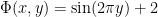
Under the assumption that ${\alpha}$ has bounded type, Kanigowski and Forni have proved quantitative mixing.

7.3. Idea of proof

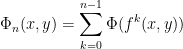
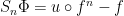
We start from a Furstenberg skew-product ${f_{\alpha,0}}$ and play with roof functions. We use again mixing by shearing. We consider intervals in the fiber (i.e. in the ${y}$ direction). We shall see that many of them shear in the flow ( ${z}$ ) direction. But there are intervals which do not shear or shear in the other direction.

7.4. Special flow dynamics

Given a point ${(x,y)}$ in the torus and ${t>0}$ , we compute ${f^\Phi_t(x,y)}$ . When ${t}$ is large, we join bottom to roof several times. Let

$\displaystyle \Phi_n(x,y)=\sum_{k=0}^{n-1}\Phi(f^k(x,y))$

and

$\displaystyle n_t(x,y):=\max\{n\,;\,\Phi_x(x,y)<t\}.$

Then

$\displaystyle f^\Phi_t(x,y)=(f^{n_t(x,y)}(x,y),t-\Phi_{n_t(x,y)}(x,y)).$

In order to exhibit shearing, we want to see how this changes in ${y}$ . Since ${f}$ is an isometry in the ${y}$ -direction, the ${y}$ -derivative of the sum ${\Phi_n}$ is the sum of ${y}$ -derivatives, i.e.

$\displaystyle \frac{\partial\Phi_n}{\partial y}=(\frac{\partial\Phi}{\partial y})_n.$

Take ${\mathcal{R}=}$ trigonometric polynomials on the torus, which are positive.

Given ${\Phi\in\mathcal{R}}$ , let ${\phi=\Phi}$ minus its average on the ${y}$ -fiber. Define ${\mathcal{M}_f}$ as the set of ${\Phi}$ such that ${\phi}$ is not a measurable coboundary.

Step 1. Since ${\phi}$ is not a measurable coboundary, the sums ${\phi_n}$ must grow,

$\displaystyle \forall C>0,\quad \mathrm{Lebesgue}(\{(x,y)\,;\,|\phi_n|(x,y)>C\})\rightarrow 1.$

This relies on a result by Gottschalk-Hedlund, plus decoupling.

Step 2. The sums ${\phi_n}$ are trigonometric polynomials of bounded degree. It follows that

$\displaystyle \forall C>0,\quad \mathrm{Lebesgue}(\{(x,y)\,;\,|\frac{\partial\phi_n}{\partial y}|(x,y)>C\})\rightarrow 1.$

There can be flat intervals where no stretch occur, so one must throw them away. But the larger ${t}$ , the shorter these intervals are.

Step 3. We use a polynomial bound on level sets of trigonometric polynomials.

The next class will deal with renormalization, deviations of ergodic averages. Only later shall we get back to Katok’s characterization of smoothly trivial special flows and to nilflows.

8. Short recap

Parabolicity is (a bit heuristically) defined by slow butterfly effect. This can be formalized for smooth flows, in terms of growth of derivatives under iteration. It is not that easy to build examples.

Presently, parabolic flows is the following list of examples,

Horocycle flows of compact constant curvature surfaces.
Unipotent flows (a generalization of the above).
Nilflows and their time-changes.
Smooth area-preserving flows.
Linear flows on flat surfaces with conical singularites.

The two first are uniformly parabolic. The next is partially parabolic. The fourth is nonuniformly parabolic, the last is elliptic with singularities.

We have proven mixing via the technique of shearing.

Here is a further example where this technique works, due to B. Fayad, of an elliptic flavour. Start with a linear flow on the ${n}$ -torus. If ${n\geq 3}$ , Fayad has been able to construct anaytic time-changes which are mixing.

Such examples are very rare (they rely on parameters being very Liouville numbers).

9. Renormalization

The word here is taken in a meaning which differs from its use in holomorphic dynamics (not to speak of quantum mechanics).

The idea is to analyze systems which are approximately self-similar, and exhibit several time scales.

We introduce the renormalization flow ${\mathcal{R}_t}$ which rescales: long trajectories become short. Given a map ${T}$ , one way to zoom in is to restrict ${T}$ to a subspace ${Y\subset X}$ and replace ${T}$ with the first return map to ${Y}$ . Eventually rescale space afterwards. But there are other means.

9.1. A series of examples

Example. Start with the horocycle flow ${h_{\mathbb R}}$ . The key relation is

$\displaystyle g_t h_s = h_{e^{t}s} g_t.$

Applying the geodesic flow to a length ${e^t}$ trajectory ${\gamma_{e^t}}$ , we get a trajectory of length ${1}$ . So the geodesic flow achieves renormalization, on the same space, with no effort.

Example. The cat map ${\psi_A}$ associated with the matrix ${A=\begin{pmatrix} 2 & 1 \ 1 & 1 \end{pmatrix}}$ on the ${2}$ -torus. Let ${\lambda_1>1}$ , ${\lambda_2<1}$ denote the eigenvalues, ${v_1,v_2}$ the eigenvectors. Let ${\phi_{\mathbb R}}$ be the linear flow in direction ${v_1}$ , with unit speed. This is an elliptic flow.

Put ${T_n=\lambda_1^n}$ . Let

$\displaystyle \gamma_{T_n}=\{\phi_t(x)\,;\,0\le t<T_n \}.$

Put ${\mathcal{R}=\psi_A^{-1}}$ . Then ${\mathcal{R}}$ maps ${\gamma_{T_n}}$ to a trajectory of ${\phi_{\mathbb R}}$ of length ${1}$ .

Express ${\psi_A}$ as the composition of two Dehn twists,

$\displaystyle A=\begin{pmatrix} 2 & 1 \\ 1 & 1 \end{pmatrix}=\begin{pmatrix} 1 & 1 \\ 0 & 1 \end{pmatrix}\begin{pmatrix} 1 & 0 \\ 1 & 1 \end{pmatrix}.$

Rotate coordinates so that eigenvector ${v_1}$ becomes vertical. Then ${\mathcal{R}}$ acts by a diagonal matrix in ${SL_2({\mathbb R})}$ , which was denoted by ${g_t}$ , ${e^t=\lambda_1}$ earlier.

Example. Higher genus toy model.

View a genus ${2}$ surface ${S}$ as a regular octagon in the Euclidean plane with edge identifications. Fix a direction ${\theta}$ , consider the linear flow in direction ${\theta}$ . It descends to a flow ${\phi_{\mathbb R}}$ on the surface which is not well-defined at the vertex

This generalizes to translation surfaces, made of a disjoint union of polygons, with identifications given by translations. The notion of a direction ${\theta}$ is well-defined on the surface (except at finally many singularities), whence a flow ${\phi_{\mathbb R}}$ with singularities.

Consider matrix

$\displaystyle P^+=\begin{pmatrix} 1 & 2(1+\sqrt{2}) \\ 0 & 1 \end{pmatrix}.$

It applies a shear on the original regular octagon. Since ${1(1+\sqrt{2})=2\cot(\frac{\pi}{8})}$ , This linear map induces a homeomorphism of the surface ${S}$ . Let us repeat in different direction (rotation by 45 degrees), get matrix ${P^-}$ . Let ${A=P^+P^-}$ , this is a hyperbolic matrix with eigenvalues ${\lambda_1>1>\lambda_2}$ . We get again an affine automorphism ${\psi_A}$ of the surface. Let ${\phi_{\mathbb R}}$ denote the linear flow in the direction of the eigenvector ${v_1}$ . Then

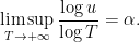
B. Veech has shown that the affine group of the surface is generated by ${\psi_A}$ and the order ${8}$ rotation. This is as large as the affine group of a translation surface can be. Therefore, ${S}$ is clled the Veech surface.

For almost every direction ${\theta}$ (the condition is that ${\tan(\theta)\notin{\mathbb Q}(\sqrt{2})}$ ), there exists a sequence of hyperbolic automorphisms ${\psi_n}$ with unstable direction ${\theta_n}$ that converge to ${\theta}$ . ${\psi_n}$ can be used to renormalize ${\phi^\theta_{\mathbb R}}$ .

Example.

For a slightly deformed octagon ${O'}$ , the affine group of the corresponding surface ${S'}$ is trivial. Nevertheless, almost every linear flow ${\phi^\theta_{\mathbb R}}$ is still renormalizable: there is a sequence of surfaces ${S_n}$ and affine hyperbolic morphisms ${\psi_n:S'\rightarrow S_n}$ with expanding direction ${\theta_n}$ converging to ${\theta}$ .

Indeed, consider the space ${\mathcal{C}}$ of linear flows on translation surfaces of genus ${2}$ . The flow of diagonal matrices acts on this space, generating a flow ${\mathcal{R}_{\mathbb R}}$ on ${\mathcal{C}}$ , known as the Teichmüller flow.

Theorem 12 (Masur-Veech) ${\mathcal{R}_{\mathbb R}}$ is recurrent.

Therefore for almost every linear flow, there exists a sequance ${t_n\rightarrow\infty}$ such that ${\mathcal{R}_{t_n}(S,\theta)}$ tends to ${(S,\theta)}$ .

9.2. What is renormalization good for?

It is used to put diophantine conditions on linear flows in higher genus. See my ICM 2022 talk (watch it on line on july 11th). I do not pursue this topic further.

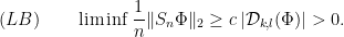
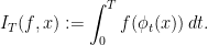
It is used to study deviations of ergodic averages. Assume a flow ${\phi_{\mathbb R}}$ is uniquely ergodic. Ergodic integrals take the form

$\displaystyle I_T(f,x):=\int_0^T f(\phi_t(x))\,dt.$

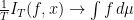
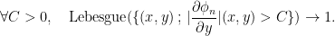
By the ergodic theorem, ${\frac{1}{T}I_T(f,x)\rightarrow\int f\,d\mu}$ for every ${x}$ . Let us focus on our favourite example, the Veech surface. The invariant measure is area in the plane. Unique ergodicity is a theorem of Masur, Kerckhoff-Masur-Smillie

We show that for functions with vanishing average,

$\displaystyle I_T(f,x)=O(T^\alpha),$

for some ${0<\alpha<1}$ (discovered by Zorich, conjectured by Kontsevitch-Zorich, proven by Forni).

Fix a basis ${\tilde\gamma_1,\ldots;\tilde\gamma_4}$ of ${H_1(S,{\mathbb Z})}$ . Fix a section ${\Sigma}$ of the linear flow. Take trajectories ${\gamma_1,\ldots,\gamma_4}$ from ${\Sigma}$ and to their first return to ${\Sigma}$ . Closing them by segments of sigma gives representatives of the basis of homology. Let

$\displaystyle \gamma_i^{n}=\psi_A^n(\gamma_i).$

Let ${B\in \mathrm{Sp}(4,{\mathbb Z})}$ be the matrix expressing the homology basis ${\psi_A(\tilde\gamma_1,\ldots,\tilde\gamma_4)}$ is the initial basis. Let ${\lambda_1>\lambda_2>1>\lambda_3=1/\lambda_2 > \lambda_4=1/\lambda_1}$ denote the eigenvalues of ${B}$ . By continuity of ${f}$ , up to a small error,

$\displaystyle \int_{0}^{\mathrm{length}(\gamma_{j}^{n})}f(\phi_t(x))\,dt=\int_{\gamma_{j}^{n}}f.$

Let us start from a large ${n_0}$ instead of ${0}$ ,

$\displaystyle \int_{\gamma_{i}^{n}}f=\sum_{j} B^{n-n_0}_{ij}\int_{\gamma_{j}^{n_0}}f:=(B^n \rho)_i.$

For simplicity, let us assume that ${\rho}$ is the eigenvector ${v_1}$ . Then

$\displaystyle \int_{\gamma_{i}^{n}}f\ge\min \{|v_1|,\|B^n\|\},$

a contradiction. Therefore ${\rho}$ must be a combination of ${v_2,v_3,v_4}$ . Thus

$\displaystyle |\int_{\gamma_{i}^{n}}f|\le\|B^n\rho\|\le \lambda_2^n.$

On the other hand, ${T=\mathrm{length}(\gamma_{j}^{n})}$ grows like ${\lambda_1^n}$ . Let ${\alpha}$ satisfy

$\displaystyle \lambda_1^\alpha=\lambda_2.$

Then ${I_T(f,x)=O(T^\alpha)}$ , as announced.

Of course, I cheated a bit, some more regularity of ${f}$ is needed.

In that example, the fact that ${\lambda_1\not=\lambda_2}$ can be explicitly. Tomorrow, I will mention results on this for general translation surfaces.

And then, back to nilflows.

9.3. Area preserving flows on surfaces

${S}$ compact connected oriented surface of genus ${g>1}$ . Let ${\phi_{\mathbb R}}$ be a flow which preserves a smooth measure ${\mu}$ . Note that ${\phi_{\mathbb R}}$ has fixed points, which are all of saddle type. In the next theorem, the number and types of fixed points are fixed.

Theorem 13 (Zorich, Forni, Avila-Viana) There exists ${g}$ distinct positive exponents ${1=\alpha_1 >\cdots>\alpha_g>0}$ such that almost every choice of ${\phi_{\mathbb R}}$ (Katok’s fundamental class, described in terms of periods) is uniquely ergodic, and for all smooth functions ${f}$ ,

$\displaystyle I_T(f,x)=(\int f\,d\mu)T+\mathcal{D}_2(f)O(T^{\alpha_2})+\cdots+\mathcal{D}_g(f)O(T^{\alpha_g})+ O(T^\epsilon),$ for all ${\epsilon>0}$ .

In this statement, ${O(T^\alpha)}$ means a function ${u}$ such that

$\displaystyle \limsup_{T\rightarrow+\infty}\frac{\log u}{\log T}=\alpha.$

Furthermore, ${\mathcal{D}_j}$ is a distribution on ${S}$ , and ${\mathcal{D}_2(f)\not=0}$ .

This type of behavior is called a power deviation spectrum. It was conjectured by Kontsevitch and Zorich, then proved by Zorich in 1997 for special functions ${f}$ , with only one term ${\alpha_2}$ . Then Forni obtained a proof in 2002 for functions with support away from fixed points, up to distinctness of exponents which was proven by Avila-Viana. Bufetov gave a more precise version, transforming the result into an asymptotic expansion. With Fraczek, we gave a different proof based on Marmi-Moussa-Yoccoz). Finally, Fraczek-Kim could handle generic saddles. The expansion then involves extra terms depending on saddles (and not on ${f}$ ).

9.4. Idea of proof

Choose coordinates such that ${\Phi_{\mathbb R}}$ appears as a time-change of a linear flow on a translation surface. The time change is smooth only away from fixed points. If function ${f}$ has support away from fixed points, one is reduced to study deviation for linear flows. For a general linear flow, a renormalization is given by a sequence of matrices ${B_n\in Sp(2g,{\mathbb Z})}$ , the Kontsevitch-Zorich cocycle. Eigenvalues are replaced with ratios of Lyapunov exponents.

10. More on renormalization

10.1. Back to nilflows

Let ${ASl(2,{\mathbb R})}$ denote the stabilizer of vector ${(1,0,0)}$ is ${Sl(3,{\mathbb R})}$ . Defined ${\mathcal{R}_t}$ by

$\displaystyle X\mapsto e^{-t}X,\quad Y\mapsto e^t Y,\quad Z\mapsto Z.$

Then ${\mathcal{R}_t}$ is recurrent, its has been used as a renormalization by Flaminio-Forni, in order to prove polynomial deviations of ergodic averages.

10.2. Renormalizable parabolic flows

Horocycle flows: yes.

Unipotent flows: unknown.

Heisenberg nilflows: yes.

Higher step nilflows: unknown in general. Special case (special flows over skew products) studied by Flaminio-Forni. In that case, the maps ${\mathcal{R}_t}$ diverge.

Linear flows over higher genus surfaces (they are smooth and area-preserving).

More general smooth flows on surfaces (not necessarily area preserving). Then ${\mathcal{R}_t}$ typically diverges. This is related to generalized interval exchange transformations.

11. Isomorphisms between time-changes

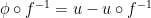
Recall that a time-change ${\tilde\phi_{\mathbb R}}$ of a flow ${\phi_{\mathbb R}}$ is

$\displaystyle \tilde\phi_t(x)=\phi_{\tau(x,t)}(x).$

When do such a change lead to a genuinely different, nonisomorphic flow?

11.1. Setting of special flows

Let ${f:Y\rightarrow Y}$ be a map. Given a roof function $latex {\Phi:Y\rightarrow{\mathbb R}_{>0}}&fg=000000$, the flow of translations on ${Y\times{\mathbb R}}$ descends to a flow $latex {\psi^{f,\Phi}_{\mathbb R}}&fg=000000$ on the quotient space

$\displaystyle X=(Y\times{\mathbb R})/\sim, \quad \text{where}\quad (y,z)\sim(f(y),z+\Phi(y).$

Lemma 14 Let ${\psi_1,\psi_2}$ be special flows over the same map ${f}$ , under roofs ${\Phi^1}$ and ${\Phi^2}$ . If there exists a function ${u:Y\rightarrow{\mathbb R}}$ such that

$\displaystyle \Phi^2=\Phi^1+u\circ f-u,$ then the two special flows are isomorphic.

Indeed, look for a conjugating homeomorphism of the form

$\displaystyle (y,z)\mapsto (y,z+u(y)).$

It commutes with translations and maps one equivalence relation to the other.

11.2. Cohomological equations

The operator ${u\mapsto u\circ f-u}$ is called the coboundary operator. Hence the equation ${u\circ f-u=\Phi}$ with unknown ${u}$ is called a cohomological equation. It sometimes appears with a twist: ${\lambda u\circ f-u=\Phi}$ , for some ${\lambda\in{\mathbb R}}$ .

There are obvious obstructions.

If ${x}$ is a periodic point, i.e. ${f^n(x)=x}$ , then

$\displaystyle \sum_{k=0}^{n-1}\Phi(f^k(x))=0.$

So every periodic orbit gives an obstruction. If ${f}$ is hyperbolic, it is essentially the only one.

More generally, if ${\mu}$ is an invariant measure, then

$\displaystyle \int \Phi\,d\mu=0.$

So every invariant measure gives an obstruction.

11.3. An elliptic example

If ${f}$ is elliptic, this is sometimes sufficient, e.g. for circle rotations ${R_\alpha}$ : if ${\Phi}$ is a trigonometric polynomial and ${\int \Phi(x)\,dx=0}$ , then there exists a solution ${u}$ . If ${\Phi}$ is smooth, a Diophantine condition on ${\alpha}$ is required in addition for the solution ${u}$ to be smooth. Indeed, in Fourier, if

$\displaystyle \Phi(x)=\sum_{k\in{\mathbb Z}}\Phi_k e^{2\pi ikx}, \quad \Phi_0=0,\quad u(x)=\sum_{k\in{\mathbb Z}}u_k e^{2\pi ikx},$

then

$\displaystyle u_k=\frac{\Phi_k}{e^{2\pi ik\alpha}-1}.$

For ${u_k}$ to decay superpolynomially, one needs that

$\displaystyle |e^{2\pi ik\alpha}-1|\ge\frac{c}{k^\tau}$

for some ${\tau}$ , which amounts to ${\alpha}$ being badly approximable by rationals.

11.4. Parabolic case

In the parabolic world, in addition to invariant measures, invariant distributions provide further obstructions.

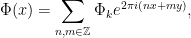
Remember that Heisenberg nilflows are special flows with constant roof over Furstenberg skew-products of the form

$\displaystyle f_{\alpha,\beta}(x,y)=(x+\alpha,y+x+\beta).$

We need study the corresponding cohomological equation.

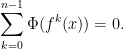
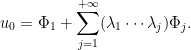
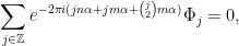
Proposition 15 In Fourier series, if

$\displaystyle \Phi(x)=\sum_{n,m\in{\mathbb Z}}\Phi_k e^{2\pi i(nx+my)},$ then the cohomological equation has a formal solution if and only if all $\displaystyle \mathcal{D}_{m,n}(\Phi)=0$ where ${\mathcal{D}_{m,n}}$ is the distribution such that $\displaystyle \mathcal{D}_{m,n}(e^{2\pi i(ax+by)}) =\begin{cases} e^{-2\pi i((\alpha n+\beta m)k+\alpha m{k\choose 2})} & \text{ if } (a,b)=(n+km,m), \\ 0 & \text{otherwise}. \end{cases}$

Indeed, let ${e_{a,b}(x,y):=e^{2\pi i(ax+by)}}$ , and

$\displaystyle u=\sum_{m,\,n\in{\mathbb Z}}u_{n,m}e_{n,m}.$

Then

$\displaystyle u\circ f =\sum_{m,\,n\in{\mathbb Z}}e^{2\pi i(n\alpha+m\beta)}.u_{n,m}e_{n+m,m}.$

The matrix ${A=\begin{pmatrix} 1 & 1 \ 0 & 1 \end{pmatrix}}$ acts on ${{\mathbb Z}^2}$ . It has a family of orbits ${{(n,0)}}$ and ${m}$ orbits

$\displaystyle O_{n,m}:=(n+m{\mathbb Z})\times\{m\},$

${0\le n<m}$ , for each ${m>0}$ . ${L^2(T^2)}$ splits accordingly, so the cohomological equation can be solved independently in each summand

$\displaystyle H_{n,m}:=\ell^2(O_{n,m}),$

and on

$\displaystyle H_0:=\ell^2({\mathbb Z}\times\{0\}).$

For ${H_0}$ , ${f}$ acts like the circle rotation ${R_\alpha}$ , so we already understand the necessary condition, given by invariant measures.

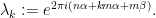
For fixed ${0\le n<m}$ and ${m>0}$ , let us denote

$\displaystyle e_k:=e_{n+km,m},\quad \Phi_k:=\Phi_{n+km,m},\quad u_k:=u_{n+km,m}.$

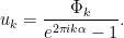
The cohomological equation reads

$\displaystyle \sum\Phi_k e_k=\sum(\lambda_{k-1}u_{k-1}-u_k),$

where

$\displaystyle \lambda_k:=e^{2\pi i(n\alpha+km\alpha+m\beta)}.$

Recursively, one gets

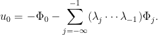
$\displaystyle u_0=-\Phi_0-\sum_{j=-\infty}^{-1}(\lambda_j\cdots\lambda_{-1})\Phi_j.$

Then

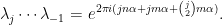
$\displaystyle \lambda_j\cdots\lambda_{-1}=e^{2\pi i(jn\alpha+jm\alpha+{j\choose 2}m\alpha)}.$

Similarly, the equation

$\displaystyle \phi\circ f^{-1}=u-u\circ f^{-1}$

yields

$\displaystyle u_0=\Phi_1+\sum_{j=1}^{+\infty}(\lambda_{1}\cdots \lambda_{j})\Phi_j.$

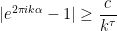
Combining both leads to

$\displaystyle \sum_{j\in{\mathbb Z}}e^{-2\pi i(jn\alpha+jm\alpha+{j\choose 2}m\alpha)}\Phi_j=0,$

i.e. ${\mathcal{D}_{n,m}(\Phi)=0}$ .

Conversely, one can see that this conditions are sufficient for existence of a formal solution, and for existence of smooth solutions under Diophantine conditions.

11.5. More general results on cohomological equations in parabolic dynamics

The case of Heisenberg nilflows, which we just treated, is due to Katok.
More general nilflows have been studied by Flaminio-Forni, as well as horocycle flows.
Linear flows on higher genus surfaces are due to Forni. In this case, one gets ${g}$ distributions ${\mathcal{D}_1,\ldots,\mathcal{D}_g}$ . If a smooth function ${f}$ is killed by all of them, ergodic integrals stay bounded. This is equivalent to ${f}$ being a coboundary, according to Gottschalk-Hedlund.

11.6. Cocycle effectiveness

Sometimes, the cohomological equation with measurable data is needed. It is much more difficult, but some miracle occurs in the parabolic setting.

Definition 16 Given a map ${f:X\rightarrow X}$ , say a function ${\Phi}$ on ${X}$ is a measurable coboundary of the exists a measurable ${u}$ such that ${u\circ f-u=\Phi}$ .

The theorem on mixing smooth time-changes of Heisenberg nilflows (Avila-Forni-Ulcigrai) required the roof not to be a measurable coboundary. It turns out that here, this is equivalent to not being a smooth coboundary.

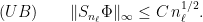
Proposition 17 Let us study the Furstenberg skew-product ${f_{\alpha,\beta}}$ on the ${2}$ -torus. Let ${\Phi}$ be a smooth function on ${T^2}$ . Then
${\Phi}$ is not a smooth coboundary ${\iff}$ ${\phi}$ is not a measurable coboundary.

Indeed, let

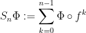
$\displaystyle S_n\Phi:=\sum_{k=0}^{n-1}\Phi\circ f^k$

denote the Birkhoff sums. Then Flaminio-Forni establish quadratic upper bounds: there exists a sequence ${n_\ell}$ such that

$\displaystyle (UB)\quad\quad \|S_{n_\ell}\Phi\|_\infty \le C\, n_\ell^{1/2}.$

Matching lower bounds exist: if ${\Phi}$ is not a smooth coboundary, there exists a nonvanishing ${\mathcal{D}_{k,l}(\Phi)}$ , and

$\displaystyle (LB) \quad\quad \liminf \frac{1}{n}\|S_n\Phi\|_2\geq c\,|\mathcal{D}_{k,l}(\Phi)|>0.$

If ${\Phi}$ is a measurable coboundary, ${\Phi=u\circ f-u}$ , then

$\displaystyle S_n\Phi =u\circ f^n -f$

stays bounded on a set of almost full measure, and grows at most quadratically on the complement. This contradicts the quadratic lower bound.

11.7. More general nilflows

Theorem 18 (Avila-Forni-Ravotti-Ulcigrai) For general nilflows of step ${k\ge 2}$ , there exists a dense (in ${C^\infty(X)}$ ) class ${\mathcal{P}}$ of generators ${\alpha}$ of time-changes, which are

either measurably trivial (i.e. measurably conjugate to the nilflow);
or mixing.

Unfortunately, the set ${\mathcal{P}}$ is not explicitly describable like in the Heisenberg case.

The proof is an induction on central extensions. It uses mixing by shearing.

12. More examples of parabolic dynamics

12.1. Parabolic perturbations which are not time-changes

These were discovered by Ravotti during his PhD at Princeton.

Here, parabolic means that the derivative of the flow grows polynomially. It implies that smooth time-changes are still parabolic.

Start with ${G=Sl(3,{\mathbb R})}$ , ${\Gamma}$ a cocompact lattice, ${X=\Gamma\setminus G}$ . Let ${h_{\mathbb R}}$ be the flow generated by a unipotent element ${U}$ . Let ${Z}$ belong to the center of the minimal unipotent and ${V}$ such that ${[U,V]=-cZ}$ .

Let ${\tilde U=U+\beta Z}$ where ${\beta}$ is a function on ${X}$ such that ${|\nabla \beta|_\infty <|c|}$ . Let ${\tilde h_{\mathbb R}}$ denote the corresponding flow.

Theorem 19 If ${\tilde h_{\mathbb R}}$ preserves a smooth measure ${\tilde\mu}$ with ${C^1}$ density, then ${\tilde h_{\mathbb R}}$ is

parabolic: ${\|\nabla\tilde h_{\mathbb R}\|=O(t^4)}$ ;
ergodic;
mixing.

Remark. Existence of ${\tilde\mu}$ ${\iff}$ there exists a time-change of the ${Z}$ -flow which commutes with ${\tilde h_{\mathbb R}}$ .

Remark. There exists such ${\tilde h_{\mathbb R}}$ which are not smoothly isomorphic to ${h_{\mathbb R}}$ . This follows from the failure of cocycle rigidity for parabolic actions, due to Wang, following many people.

Remark. Ergodicity needs be proven, it does not follow from general principles.

The proof relies on mixing by shearing, although in a setting different from what we have already met. Consider arcs of orbits of ${V}$ and push them by ${\tilde h_{\mathbb R}}$ . Since

$\displaystyle \nabla \tilde h_{\mathbb R}(V)=V+u_t(x)Z$

where ${u_t(x)}$ is an ergodic integral for ${\tilde h_{\mathbb R}}$ .

12.2. What else can shearing be used for?

A strong, quantitative, shearing can be used to establish spectral results. Here, I mean the spectrum of the Koopman operator

$\displaystyle U_t:L^2\rightarrow L^2,\quad f\mapsto f\circ\phi_t.$

To each ${f\in L^2(X,\mu)}$ , there corresponds a spectral measure ${\sigma_f}$ on ${{\mathbb R}}$ . Its Fourier coefficients are given by selfcorrelations of ${f}$ , i.e.

$\displaystyle \hat\sigma_f(t)=\langle f\circ \phi_t , f \rangle_2.$

The spectrum of ${U_t}$ is absolutely continuous ${\iff}$ for all ${f\in L^2}$ , ${\hat\sigma_f}$ is absolutely continuous ${\iff}$ for all ${f\in L^2}$ , ${\int_{{\mathbb R}}\hat\sigma_f(t)^2\,dt <+\infty}$ .

If ${\phi_{\mathbb R}}$ is ergodic, it is enough to study functions ${f}$ which are smooth coboundaries.

Theorem 20 (Forni-Ulcigrai) Smooth time-changes of a horocycle flow has absolutely continuous spectrum.

The proof uses quantitative bounds

$\displaystyle |\langle f\circ \phi_t , f \rangle_2|\le \frac{Cf}{t}.$

Since ${\frac{1}{t}\in L^2}$ , this implies absolute continuity.

Fayad-Forni-Kanigowski consider smooth area-preserving flows on the ${2}$ -torus with a stopping point.

12.3. Ratner property

M. Ratner uses a quantitative form of shearing for unipotent flows.

Shearing takes some time. Ratner requires the following:

For all ${\epsilon>0}$ , for all large enough ${t_0}$ , there exists a set ${X_\epsilon}$ of measure ${>1-\epsilon}$ , for all pairs ${x,y\in X_\epsilon}$ not in the same orbit, but such that ${d(x,y)<\epsilon}$ , there exists ${t_1>t_0}$ such that

$\displaystyle d(\phi_{t_1}(x),\phi_{t_1+s}(y))<\epsilon$

and

$\displaystyle d(\phi_\tau(\phi_{t_1}(x)),\phi_\tau(\phi_{t_1+s}(y)))<\epsilon$

for all ${\tau\in [t_1,(1+K)t_1]}$ .

For a long time, this was used only in algebraic dynamics, until a more flexible variant, called switchability, was introduced. It means that one can switch past and future.

Fayad-Kanigowski and Kanigowski-Kulaga-Ulcigrai established this variant for typical smooth area-preserving flows on surfaces. This implies mixing of all orders.

Here is another application if these ideas:

Theorem 21 (Kanigowski-Lemanczyk-Ulcigrai) For all smooth time-changes ${\tilde h_{\mathbb R}}$ of the horocycle flow, the rescaled flow ${\tilde h_{\mathbb R}^K}$ is not isomorphic to ${\tilde h_{\mathbb R}}$ .

They are actually disjoint in Furstenberg’s sense. Recall that the horocycle flow itself is isomorphic to its rescalings.

We use a disjointness criterion based on this switchable variant of Ratner’s property.

12.4. Summary

Parabolic means slow butterfly effect.
Typically slow mixing.
Slow equidistribution.
Disjointness of rescalings.
Obstructions to cohomological equation.

Tools:

Shearing.
Ratner property and switchability.
Renormalization.

	metric2011 on Notes of Sa’ar Hersonsky…
	CH on Videos
	Stefan Wenger on Notes of Stefan Wenger’s…
	Stefan Wenger on Notes of Stefan Wenger’s…
	Stefan Wenger on Notes of Stefan Wenger’s…

Notes of Corinna Ulcigrai’s Hadamard Lectures, june 2022

About metric2011

Leave a comment Cancel reply

Recent Posts

Recent Comments

Archives

Categories

Meta

Notes of Corinna Ulcigrai’s Hadamard Lectures, june 2022

Share this:

Related

About metric2011

Leave a comment Cancel reply

Recent Posts

Recent Comments

Archives

Categories

Meta