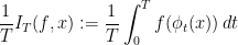
Parabolic dynamics
1. Survey
1.1. What does hyperbolic, elliptic mean in dynamics?
Let  be a dynamical system. Even if deterministic, it can exhibit a chaotic behaviour. This has several characteristics. One of them is the Butterfly effect: sensitive dependence on initial conditions (SDIC).
Definition 1 A flow  has SDIC if there exists
  such that
  ,
,  ,
,  such that
  and
and  such that
  .
.
A quantitative measurement of SDIC is provided by the dependence of  on
on  .
.
Definition 2 Let  be a nondecreasing function. A flow has SDIC of order
  if in the above definition, one can take such that
  .
.
This leads us to a rough division of dynamical systems:
- Elliptic: no SDIC, or if any, subpolynomial.
- Hyperbolic: SDIC is fast, exponential.
- Parabolic: SDIC is slow, subexponential.
This trichotomy is advertised in Katok-Hasselblatt’s book.
For instance, entropy is a measure of chaos. Elliptic or parabolic dynamical systems have zero entropy. Hyperbolic dynamical systems have positive entropy.
1.2. Examples of elliptic dynamical systems
- Circle diffeomorphisms.
- Linear flows on the torus (these two examples are related, one is the suspension of the other).
- Billiards in convex domains. Usually, there are many periodic orbits, trapping regions, caustics.
This the realm of Hamiltonian dynamics and KAM theory.
1.3. Examples of hyperbolic dynamical systems
- Automorphisms of a torus which are Anosov, i.e. all eigenvalues have absolute values
 . Then orbits diverge exponentially: if
  ,
,  , set
, set  . Then
  mod
mod  and
and  reaches
  in time
  such that
  for
for  , an exponential.
 - Geodesic flows on constant curvature surfaces.
- Sinai’s billiard: a rectangle with a circular obstacle. Somewhat equivalent to the motion of two hard spheres on a torus. Scattering occurs after hitting the obstacle, due to its strict convexity.
This is the realm of Anosov-Sinai and others’ dynamics. Structural stability occurs: hyperbolic systems form an open set.
1.4. Examples of parabolic dynamical systems
- Horocycle flows on constant curvature surfaces. They were introduced by Hedlund, followed by Dani, Furstenberg, Marcus, Ratner.
- Nilflows on nilmanifolds. If
 is a cocompact lattive in a nilpotent Lie group, let be a
  -parameter subgroup of
  acting by right translations on . It descends to
  . Both examples are algebraic, this provides us with tools to study them. They are a bit too special to illustrate parabolic dynamics.
 - Smooth area-preserving flows on higher genus surfaces.
- Ehrenfest’s billiard: rectangular, with a rectangular obstacle. Here, SDIC is only caused by discontinuities due to corners. More generally, billiards in rational polygons (angles belong to
 ), or equivalently linear flows on translation surfaces. This field is known as Teichmüller dynamics. Forni considers them as elliptic systems with singularities, I prefer to stress their parabolic character.
1.5. Uniformity
Within hyperbolic dynamics, there is a subdivision in uniformly hyperbolic, nonuniformly hyperbolic and partially hyperbolic.
In the same manner, we see horocycle flows as uniformly parabolic, and nilflows as partially parabolic, with both elliptic and parabolic directions. Area-preserving flows on surfaces have fixed points which introduce partially parabolic behaviour: shearing is uniform or not. However, there is no formal definition.
1.6. More examples of parabolic behaviours
Parabolicity is not stable. However, Ravotti has discovered a -parameter perturbation of unipotent flows in  .
.
A flow  is a time-change of a given flow
  if there exists a function
  such that

For to be a flow, it is necessary that  be a cocycle.
Both flows have the same trajectories. A feature of parabolic dynamics is that a typical time-change is not isomorphic to and has new chaotic features. Indeed, an isomorphism would solve the cohomology equation, and there are obstructions.
1.7. Program
Study smooth time-changes of algebraic flows.
Goes back to Marcus in the 1970’s. Algebraic tools break down, softer methods are required: geometric mechanisms. Also, we expect the features exhibited by time changes to be more typical.
2. Chaotic properties
2.1. Definitions
Definition 3 Let  be a measure space with finite measure. Let be a measure preserving flow. The trajectory of a point
  is equidistributed with respect to
  if for every smooth observable
  ,
,
 tends to
  as
as  tends to
  .
.
is ergodic if almost every has equidistributed orbit with respect to .
This is Boltzmann hypothesis.
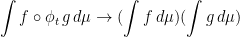
Definition 4 Say is mixing if for all  , the correlation
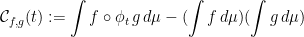 tends to as tends to .
This means decorrelation of functions. This implies ergodicity.
The speed at which decorrelation occurs is a significative feature too.
Definition 5 The speed of mixing is a function  such that for all smooth observables
  , the correlation decays at speed , i.e.
 as tends to .
2.2. Relation to the trichotomy
Elliptic systems often are not ergodic, but even when they are, they are not mixing.
Hyperbolic and parabolic systems can be mixing, but at different speeds:
- hyperbolic
 exponential decay of correlations.
 - in parabolic systems, we expect that, if mixing occurs, the decay of correlations is slower: polynomial or subpolynomial.
A related concept is that of polynomial deviations of ergodic averages: if  is smooth and has vanishing integral, s ergodic and
  is an equidistribution point,

and no faster. This phenomenon was first discovered on horocycle flows, then Teichmüller flows (Zorich, experimentally, Kontsevitch-Zorich for a proof).
2.3. Other features
Spectral properties. Let  be the operator
  on
on  . Then is unitary. What is its spectrum?
Disjointness of rescalings. Rescaling means linear time change  .
.
3. Results
Horocycle flow is mixing (Ratner). The spectrum is Lebesgue absolutely continuous.
Time changes of horocycle flows are mixing (Marcus, by shearing). This can be made quantitative (Forni-Ulcigrai).
Disjointness of rescalings fails for horocycle flows, but hold for nontrivial time changes (Kanigowski-Ulcigrai and Flaminio-Forni). The spectrum is Lebesgue absolutely continuous as well.
Nilflows themselves are not mixing, but typical time changes of nilflows are mixing (Avila-Forni-Ravotti-Ulcigrai).
We shall see geometric mechanisms at work:
- Mixing via shearing.
- Ratner property of shearing.
- Renormizable parabolic flows.
- Deviations of ergodic integrals.
4. Horocycle flows
Today’s goal is to explain the technique of mixing by shearing.
4.1. Algebraic viewpoint
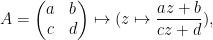
Consider  and its subgroups

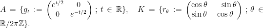
Every matrix can be uniquely written  , hence
  . The factors do not commute, because of the key relation

The key relation can be interpreted as a selfsimilarity property:  is a fixed point of renormalization by
  .
.
Take a discrete and cocompact subgroup  . Then
  and act on
  by left multiplication. The key relation implies that the rescaled flow $latex {h_{\mathbb R}^k=(h_{ks})_{s\in{\mathbb R}}}&fg=000000$ is conjugated to $latex {h_{\mathbb R}}&fg=000000$. This fails for other (nonrescaling) time changes, as I proved recently with Fraczek and Kanigowski.
4.2. Geometric viewpoint
Let  denote the upper half plane, with metric
  .
.
Fact.  acts isometrically and transitively on , and this yields a diffeomorphism of with the unit tangent bundle
  .
.
Indeed, the action is by Möbius transformations
on , and by their derivatives on .
With this identification, orbits of are curves which project to geodesics of , and coincide with their lifts by their unit speed vector. On the other hand, orbits of are curves which projects to horocycles of , and coincide with their lifts by their unit normal outward pointing vectors. Lifts by inward pointing normal vectors are orbits of  .
.
 is a hyperbolic flow: it contracts in the direction of -orbits, it dilates in the direction of -orbits,
4.3. Classical results
Let denote Haar measure on . It maps via  to hyperbolic volume. Consider the induced measure on (still denoted by ). Then
  and acts on
  by measure preserving transformations.
Then
- is ergodic (Hopf). It is far from being unique ergodic (plenty of periodic orbits).
- is mixing.
- is uniquely ergodic (Furstenberg). This means that every orbit is equidistributed with respect to .
5. Shearing
This is an alternate way to prove mixing. The idea goes back to Marcus (Annals of Math. 1977). Marcus covered a more general situation, and proved mixing of all orders (i.e. for multicorrelations, integrals involving an arbitrarily large number of functions).
Let us shift viewpoint on the key relation. Let  be a piece of -orbit of length
  . Let
. Let

Then  is sheared or tilted in the direction of the geodesic flow.
Key idea in parabolic dynamics: In several parabolic systems, the Butterfly effect happens in a special way, e.g. shearing. Points nearby move parallel, but with different speeds. This implies that transverse arcs shear.
5.1. Recipe for mixing in parabolic dynamics
Here are the ingredients:
- A uniquely ergodic flow .
- A transverse direction which is sheared in the direction of the flow.
By assumption, for every , the trajectory  equidistributes with respect to . We want to upgrade it to mixing, which is a property of sets: indeed
is equivalent to

i.e  equidistributes as
  .
.
The idea is to cover by short arcs in the transverse direction. We prove that each such arc equidistributes, and apply Fubini. I.e. if  , apply
  . Then
  .
.
Each  becomes close to a long piece of orbit of . By unique ergodicity, that piece equidistributes, and this implies equidistribution for
  .
.
5.2. Time change
Let  be a smooth time change, which is a cocycle with respect to a given smooth flow , i.e.

We are interested in the flow  defined by
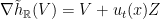
The generator of is
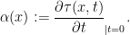
It is a smooth nonnegative function on . We assume that  . We denote by
  .
.
Remark. If is generated by a smooth vectorfield  , then is generated by the vectorfield
  .
.
Theorem 6 (Forni-Ulcigrai) Let be the horocyclic flow of a compact constant curvature surface. For any smooth function  , the flow is mixing, with quantitative estimates which imply that the spectrum is absolutely continuous with respect to Lebesgue measure.
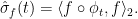
Lemma 7 Let denote the generator of and the generator of . Take a segment of -orbit
 Let
Let  Then
Then 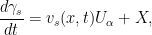 where
where 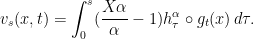
Remark.  , hence
  . Thus, as
  tends to
  ,
,  tends to a finite limit, the shear rate.
Proof of Lemma. It relies on ![{[U,X]=U}](https://s0.wp.com/latex.php?latex=%7B%5BU%2CX%5D%3DU%7D&bg=ffffff&fg=000000&s=0&c=20201002) , which implies that
, which implies that ![{[U_\alpha,X]=(\frac{X\alpha}{\alpha}-1)U_\alpha}](https://s0.wp.com/latex.php?latex=%7B%5BU_%5Calpha%2CX%5D%3D%28%5Cfrac%7BX%5Calpha%7D%7B%5Calpha%7D-1%29U_%5Calpha%7D&bg=ffffff&fg=000000&s=0&c=20201002) .
.
We see that we need compute integrals over sheared arcs  . Let be a smooth function. Then
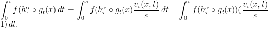
The second term is an ergodic integral which is easy to handle. The main term is the first term, which can be rewritten

where  ,
,  .
.
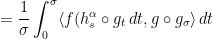
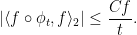
To deduce mixing, one must estimate inner products  . We integrate by parts
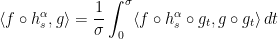
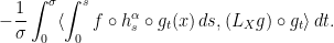
The second term is again an ergodic integral that tends to .
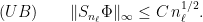
5.3. Quantitative equidistribution estimates
We are interested in ergodic integrals of the form
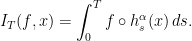
Flaminio-Forni treat the un-time-changed case  and show that
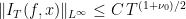
for some  . One can adapt their arguments, using estimates by Bufetov-Forni, to the time-changed case, and get similar estimates.
5.4. Additional references
Marcus original technique already proved mixing. His setting was Anosov flows, with their stable and unstable foliations. From these, a flow can be defined, which satisfies
where $latex {s^*}&fg=000000$ has a continuous mixed partial second derivative $latex {\frac{\partial s^*}{\partial t \partial s}}&fg=000000$. So we see that time-changes were already in the picture.
Kushnirenko was able to prove mixing for smooth time-changes, assuming
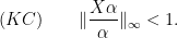
Thus small time-changes are mixing. What about larger ones? This is still open.
Tiedra de Aldecoa uses a different method to prove absolute continuity of the spectrum for time changes satisfying (KC).
Generalizations. The setting is algebraic dynamics: a unipotent -parameter subgroup acting on  , semisimple Lie group.
Lucia Simonelli (Forni’s student) could prove absolute continuity of the spectrum for time changes satisfying (KC).
Davide Ravotti (my student) could prove quantitative mixing.
Kanigowski and Ravotti could prove quantitative  -mixing.
6. Heisenberg nilfows
Let  denote the Lie group of unipotent
  matrices, with
  as standard generators of its Lie algebra,
 ![{Z=[X,Y]}](https://s0.wp.com/latex.php?latex=%7BZ%3D%5BX%2CY%5D%7D&bg=ffffff&fg=000000&s=0&c=20201002) . Let
. Let  be a discrete cocompact lattice (for instance, unipotent matrices with integer entries). We call
  the Heisenberg nilmanifold. acts on by right multiplication. The action of a -parameter subgroup is called a nilflow.
6.1. Classical results
Auslander-Green-Hahn (1963) studied unique ergodicity of nilflows. They showed that is  can be written
  , for the nilflow defined by
  ,
,
unique ergodicity  ergodicity minimality
  and are rationally independent.
Rational independence means that no linear relation with nonzero integral coefficients  can hold.
In other words, if we project the situation to the  -torus
  where
where ![{\bar H=H/[H,H]}](https://s0.wp.com/latex.php?latex=%7B%5Cbar+H%3DH%2F%5BH%2CH%5D%7D&bg=ffffff&fg=000000&s=0&c=20201002) ,
,  , then the flow
  projects to a flow
  on
on  , and
, and
unique ergodicity for unique ergodicity for  .
.
Here, we have used a theorem of Furstenberg on skew-products of rotations of the circle.
Definition 8 For real numbers  , let
, let  be the diffeomorphism of the -torus defined by

In general, a skew-product over a map  is a map
  which is fiber-preserving (with respect to the projection
  ) and the permutation of fibers is given by . In the example at hand, is isometric on fibers.
6.2. First return map
Lemma 9 Assume that the Heisenberg nilflow is uniquely ergodic. There is a transverse submanifold  , diffeomorphic to a torus, such that the Poincaré return map
  , given by
  ,
,  the first return time to
  , is one of the Furstenberg skew-products .
Proof of the Lemma. lifts to a vertical plane  in . Since and
  commute, is diffeomorphic to a torus. If is uniquely ergodic,
  , so is transverse to the flow.
We show that  is a return time. We use the fact that
  . So using the Campbell-Hausdorff-Dynkin formula, we compute

This point belongs to , so  .
.
6.3. Lack of mixing
The above Lemma shows th at we can now focus on Furstenberg skew-products. We shall see that the parameter  plays no role, so we focus on
  .
.
Definition 10 Given a map  and a function
  (called the roof function), we define the special flow
  over under
  as follows: it is a flow on an -bundle
  over the circle, the quotient of the vertical unit speed flow on
  under the identification
Fact. If a flow  admits a global Poincaré section with first return time , then is isomorphic to the special flow of the first return map with roof function .
In the case at hand, the roof function is constant. Therefore, the special flow is not mixing: if  ,
,  a short interval, so do its images by the vertical unit speed flow, and so do their projections to , which are the images of a set
  and its images by the special flow.
This shows that Heisenberg nilflows are never mixing.
7. Mixing time-changes
The following contents can be found in Avila-Forni-Ulcigrai. A recent generalization to all step 2 nilflows can be found in Avila-Forni-Ravotti-Ulcigrai. Ravotti has treated filiform nilflows.
Let be a Heisenberg nilflow and a smooth positive function on . Let
Then the time-change is given by

7.1. Time-changes versus special flows
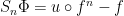
We have seen that Heisenberg nilflows are special flows with constant roof function. The time-change  is again a special flow, over the same skew-product, but with roof function
7.2. Trivial time-changes
Beware that there exist smooth time-changes which are trivial, i.e. smoothly conjugate to the original nilflow.
In general, adding a coboundary  to the roof function of a special flow produces an isomorphic flow. This leads us to the following problem: understand cohomology of nilflows. Here are our ultimate results.
Theorem 11 Let be a There exists a dense set  in
in  of roof functions, and a vectorspace
  of countable dimension and codimension, such that if a roof function is chosen in
  , the corresponding special flow
  is mixing.
Moreover, for  ,
,

In fact, Katok has found a nice characterization of which are smoothly trivial. I will come back to this next week. Today, I merely give one example.
Example.  is a smoothly trivial roof function.
Under the assumption that has bounded type, Kanigowski and Forni have proved quantitative mixing.
7.3. Idea of proof
We start from a Furstenberg skew-product and play with roof functions. We use again mixing by shearing. We consider intervals in the fiber (i.e. in the  direction). We shall see that many of them shear in the flow (
 ) direction. But there are intervals which do not shear or shear in the other direction.
7.4. Special flow dynamics
Given a point  in the torus and
  , we compute
  . When is large, we join bottom to roof several times. Let
and

Then

In order to exhibit shearing, we want to see how this changes in . Since is an isometry in the -direction, the -derivative of the sum  is the sum of -derivatives, i.e.
Take  trigonometric polynomials on the torus, which are positive.
Given , let  minus its average on the -fiber. Define
  as the set of such that
  is not a measurable coboundary.
Step 1. Since is not a measurable coboundary, the sums  must grow,

This relies on a result by Gottschalk-Hedlund, plus decoupling.
Step 2. The sums are trigonometric polynomials of bounded degree. It follows that
There can be flat intervals where no stretch occur, so one must throw them away. But the larger , the shorter these intervals are.
Step 3. We use a polynomial bound on level sets of trigonometric polynomials.
The next class will deal with renormalization, deviations of ergodic averages. Only later shall we get back to Katok’s characterization of smoothly trivial special flows and to nilflows.
8. Short recap
Parabolicity is (a bit heuristically) defined by slow butterfly effect. This can be formalized for smooth flows, in terms of growth of derivatives under iteration. It is not that easy to build examples.
Presently, parabolic flows is the following list of examples,
- Horocycle flows of compact constant curvature surfaces.
- Unipotent flows (a generalization of the above).
- Nilflows and their time-changes.
- Smooth area-preserving flows.
- Linear flows on flat surfaces with conical singularites.
The two first are uniformly parabolic. The next is partially parabolic. The fourth is nonuniformly parabolic, the last is elliptic with singularities.
We have proven mixing via the technique of shearing.
Here is a further example where this technique works, due to B. Fayad, of an elliptic flavour. Start with a linear flow on the -torus. If  , Fayad has been able to construct anaytic time-changes which are mixing.
Such examples are very rare (they rely on parameters being very Liouville numbers).
9. Renormalization
The word here is taken in a meaning which differs from its use in holomorphic dynamics (not to speak of quantum mechanics).
The idea is to analyze systems which are approximately self-similar, and exhibit several time scales.
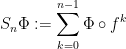
We introduce the renormalization flow  which rescales: long trajectories become short. Given a map , one way to zoom in is to restrict to a subspace
  and replace with the first return map to . Eventually rescale space afterwards. But there are other means.
9.1. A series of examples
Example. Start with the horocycle flow . The key relation is
Applying the geodesic flow to a length  trajectory
  , we get a trajectory of length . So the geodesic flow achieves renormalization, on the same space, with no effort.
Example. The cat map  associated with the matrix
  on the -torus. Let
  ,
,  denote the eigenvalues,
  the eigenvectors. Let be the linear flow in direction
  , with unit speed. This is an elliptic flow.
Put  . Let
. Let

Put  . Then maps
  to a trajectory of of length .
Express as the composition of two Dehn twists,
Rotate coordinates so that eigenvector becomes vertical. Then acts by a diagonal matrix in  , which was denoted by
  ,
,  earlier.
Example. Higher genus toy model.
View a genus surface as a regular octagon in the Euclidean plane with edge identifications. Fix a direction  , consider the linear flow in direction . It descends to a flow on the surface which is not well-defined at the vertex
This generalizes to translation surfaces, made of a disjoint union of polygons, with identifications given by translations. The notion of a direction is well-defined on the surface (except at finally many singularities), whence a flow with singularities.
Consider matrix
It applies a shear on the original regular octagon. Since  , This linear map induces a homeomorphism of the surface . Let us repeat in different direction (rotation by 45 degrees), get matrix
  . Let
. Let  , this is a hyperbolic matrix with eigenvalues
  . We get again an affine automorphism of the surface. Let denote the linear flow in the direction of the eigenvector . Then
B. Veech has shown that the affine group of the surface is generated by and the order  rotation. This is as large as the affine group of a translation surface can be. Therefore, is clled the Veech surface.
For almost every direction (the condition is that  ), there exists a sequence of hyperbolic automorphisms
  with unstable direction
  that converge to . can be used to renormalize
  .
.
Example.
For a slightly deformed octagon  , the affine group of the corresponding surface
  is trivial. Nevertheless, almost every linear flow is still renormalizable: there is a sequence of surfaces
  and affine hyperbolic morphisms
  with expanding direction converging to .
Indeed, consider the space  of linear flows on translation surfaces of genus . The flow of diagonal matrices acts on this space, generating a flow
  on , known as the Teichmüller flow.
Theorem 12 (Masur-Veech) is recurrent.
Therefore for almost every linear flow, there exists a sequance  such that
  tends to
  .
.
9.2. What is renormalization good for?
It is used to put diophantine conditions on linear flows in higher genus. See my ICM 2022 talk (watch it on line on july 11th). I do not pursue this topic further.
It is used to study deviations of ergodic averages. Assume a flow is uniquely ergodic. Ergodic integrals take the form
By the ergodic theorem,  for every . Let us focus on our favourite example, the Veech surface. The invariant measure is area in the plane. Unique ergodicity is a theorem of Masur, Kerckhoff-Masur-Smillie
We show that for functions with vanishing average,
for some  (discovered by Zorich, conjectured by Kontsevitch-Zorich, proven by Forni).
Fix a basis  of
of  . Fix a section of the linear flow. Take trajectories
  from and to their first return to . Closing them by segments of sigma gives representatives of the basis of homology. Let

Let  be the matrix expressing the homology basis
  is the initial basis. Let
  denote the eigenvalues of
  . By continuity of , up to a small error,
Let us start from a large  instead of ,
For simplicity, let us assume that  is the eigenvector . Then
a contradiction. Therefore must be a combination of  . Thus
On the other hand,  grows like
  . Let satisfy

Then  , as announced.
Of course, I cheated a bit, some more regularity of is needed.
In that example, the fact that  can be explicitly. Tomorrow, I will mention results on this for general translation surfaces.
And then, back to nilflows.
9.3. Area preserving flows on surfaces
compact connected oriented surface of genus  . Let be a flow which preserves a smooth measure . Note that has fixed points, which are all of saddle type. In the next theorem, the number and types of fixed points are fixed.
Theorem 13 (Zorich, Forni, Avila-Viana) There exists  distinct positive exponents
  such that almost every choice of (Katok’s fundamental class, described in terms of periods) is uniquely ergodic, and for all smooth functions ,
 for all
  .
.
In this statement,  means a function
  such that
Furthermore,  is a distribution on , and
  .
.
This type of behavior is called a power deviation spectrum. It was conjectured by Kontsevitch and Zorich, then proved by Zorich in 1997 for special functions , with only one term  . Then Forni obtained a proof in 2002 for functions with support away from fixed points, up to distinctness of exponents which was proven by Avila-Viana. Bufetov gave a more precise version, transforming the result into an asymptotic expansion. With Fraczek, we gave a different proof based on Marmi-Moussa-Yoccoz). Finally, Fraczek-Kim could handle generic saddles. The expansion then involves extra terms depending on saddles (and not on ).
9.4. Idea of proof
Choose coordinates such that  appears as a time-change of a linear flow on a translation surface. The time change is smooth only away from fixed points. If function has support away from fixed points, one is reduced to study deviation for linear flows. For a general linear flow, a renormalization is given by a sequence of matrices
  , the Kontsevitch-Zorich cocycle. Eigenvalues are replaced with ratios of Lyapunov exponents.
10. More on renormalization
10.1. Back to nilflows
Let  denote the stabilizer of vector
  is
is  . Defined by

Then is recurrent, its has been used as a renormalization by Flaminio-Forni, in order to prove polynomial deviations of ergodic averages.
10.2. Renormalizable parabolic flows
Horocycle flows: yes.
Unipotent flows: unknown.
Heisenberg nilflows: yes.
Higher step nilflows: unknown in general. Special case (special flows over skew products) studied by Flaminio-Forni. In that case, the maps diverge.
Linear flows over higher genus surfaces (they are smooth and area-preserving).
More general smooth flows on surfaces (not necessarily area preserving). Then typically diverges. This is related to generalized interval exchange transformations.
11. Isomorphisms between time-changes
Recall that a time-change  of a flow is
When do such a change lead to a genuinely different, nonisomorphic flow?
11.1. Setting of special flows
Let  be a map. Given a roof function $latex {\Phi:Y\rightarrow{\mathbb R}_{>0}}&fg=000000$, the flow of translations on
  descends to a flow $latex {\psi^{f,\Phi}_{\mathbb R}}&fg=000000$ on the quotient space

Lemma 14 Let  be special flows over the same map , under roofs
  and
and  . If there exists a function
  such that
 then the two special flows are isomorphic.
Indeed, look for a conjugating homeomorphism of the form
It commutes with translations and maps one equivalence relation to the other.
11.2. Cohomological equations
The operator  is called the coboundary operator. Hence the equation
  with unknown is called a cohomological equation. It sometimes appears with a twist:
  , for some
  .
.
There are obvious obstructions.
If is a periodic point, i.e.  , then
So every periodic orbit gives an obstruction. If is hyperbolic, it is essentially the only one.
More generally, if is an invariant measure, then

So every invariant measure gives an obstruction.
11.3. An elliptic example
If is elliptic, this is sometimes sufficient, e.g. for circle rotations  : if is a trigonometric polynomial and
  , then there exists a solution . If is smooth, a Diophantine condition on is required in addition for the solution to be smooth. Indeed, in Fourier, if

then
For  to decay superpolynomially, one needs that
for some , which amounts to being badly approximable by rationals.
11.4. Parabolic case
In the parabolic world, in addition to invariant measures, invariant distributions provide further obstructions.
Remember that Heisenberg nilflows are special flows with constant roof over Furstenberg skew-products of the form

We need study the corresponding cohomological equation.
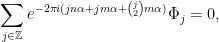
Proposition 15 In Fourier series, if
 then the cohomological equation has a formal solution if and only if all
  where
where  is the distribution such that
Indeed, let  , and
, and
Then
The matrix  acts on . It has a family of orbits
  and
and  orbits
 , for each
  .
.  splits accordingly, so the cohomological equation can be solved independently in each summand
and on
For  , acts like the circle rotation , so we already understand the necessary condition, given by invariant measures.
For fixed and , let us denote

The cohomological equation reads

where
Recursively, one gets
Then
Similarly, the equation
yields
Combining both leads to
i.e.  .
.
Conversely, one can see that this conditions are sufficient for existence of a formal solution, and for existence of smooth solutions under Diophantine conditions.
11.5. More general results on cohomological equations in parabolic dynamics
- The case of Heisenberg nilflows, which we just treated, is due to Katok.
- More general nilflows have been studied by Flaminio-Forni, as well as horocycle flows.
- Linear flows on higher genus surfaces are due to Forni. In this case, one gets distributions
 . If a smooth function is killed by all of them, ergodic integrals stay bounded. This is equivalent to being a coboundary, according to Gottschalk-Hedlund.
11.6. Cocycle effectiveness
Sometimes, the cohomological equation with measurable data is needed. It is much more difficult, but some miracle occurs in the parabolic setting.
Definition 16 Given a map , say a function on is a measurable coboundary of the exists a measurable such that .
The theorem on mixing smooth time-changes of Heisenberg nilflows (Avila-Forni-Ulcigrai) required the roof not to be a measurable coboundary. It turns out that here, this is equivalent to not being a smooth coboundary.
Proposition 17 Let us study the Furstenberg skew-product on the -torus. Let be a smooth function on  . Then
is not a smooth coboundary  is not a measurable coboundary.
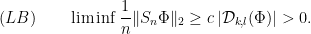
Indeed, let
denote the Birkhoff sums. Then Flaminio-Forni establish quadratic upper bounds: there exists a sequence  such that
Matching lower bounds exist: if is not a smooth coboundary, there exists a nonvanishing  , and
, and
If is a measurable coboundary,  , then
stays bounded on a set of almost full measure, and grows at most quadratically on the complement. This contradicts the quadratic lower bound.
11.7. More general nilflows
Theorem 18 (Avila-Forni-Ravotti-Ulcigrai) For general nilflows of step  , there exists a dense (in
  ) class
  of generators of time-changes, which are
- either measurably trivial (i.e. measurably conjugate to the nilflow);
- or mixing.
Unfortunately, the set is not explicitly describable like in the Heisenberg case.
The proof is an induction on central extensions. It uses mixing by shearing.
12. More examples of parabolic dynamics
12.1. Parabolic perturbations which are not time-changes
These were discovered by Ravotti during his PhD at Princeton.
Here, parabolic means that the derivative of the flow grows polynomially. It implies that smooth time-changes are still parabolic.
Start with  ,
,  a cocompact lattice,
  . Let be the flow generated by a unipotent element . Let belong to the center of the minimal unipotent and
  such that
 ![{[U,V]=-cZ}](https://s0.wp.com/latex.php?latex=%7B%5BU%2CV%5D%3D-cZ%7D&bg=ffffff&fg=000000&s=0&c=20201002) .
.
Let  where is a function on such that
  . Let denote the corresponding flow.
Theorem 19 If preserves a smooth measure  with
with  density, then is
- parabolic:
 ;
; - ergodic;
- mixing.
Remark. Existence of there exists a time-change of the -flow which commutes with .
Remark. There exists such which are not smoothly isomorphic to . This follows from the failure of cocycle rigidity for parabolic actions, due to Wang, following many people.
Remark. Ergodicity needs be proven, it does not follow from general principles.
The proof relies on mixing by shearing, although in a setting different from what we have already met. Consider arcs of orbits of and push them by . Since
where  is an ergodic integral for .
12.2. What else can shearing be used for?
A strong, quantitative, shearing can be used to establish spectral results. Here, I mean the spectrum of the Koopman operator

To each  , there corresponds a spectral measure
  on
on  . Its Fourier coefficients are given by selfcorrelations of , i.e.
The spectrum of is absolutely continuous for all  ,
,  is absolutely continuous for all ,
  .
.
If is ergodic, it is enough to study functions which are smooth coboundaries.
Theorem 20 (Forni-Ulcigrai) Smooth time-changes of a horocycle flow has absolutely continuous spectrum.
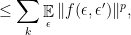
The proof uses quantitative bounds
Since  , this implies absolute continuity.
Fayad-Forni-Kanigowski consider smooth area-preserving flows on the -torus with a stopping point.
12.3. Ratner property
M. Ratner uses a quantitative form of shearing for unipotent flows.
Shearing takes some time. Ratner requires the following:
For all , for all large enough  , there exists a set
  of measure
  , for all pairs
  not in the same orbit, but such that , there exists
  such that
and

for all ![{\tau\in [t_1,(1+K)t_1]}](https://s0.wp.com/latex.php?latex=%7B%5Ctau%5Cin+%5Bt_1%2C%281%2BK%29t_1%5D%7D&bg=ffffff&fg=000000&s=0&c=20201002) .
.
For a long time, this was used only in algebraic dynamics, until a more flexible variant, called switchability, was introduced. It means that one can switch past and future.
Fayad-Kanigowski and Kanigowski-Kulaga-Ulcigrai established this variant for typical smooth area-preserving flows on surfaces. This implies mixing of all orders.
Here is another application if these ideas:
Theorem 21 (Kanigowski-Lemanczyk-Ulcigrai) For all smooth time-changes of the horocycle flow, the rescaled flow  is not isomorphic to .
They are actually disjoint in Furstenberg’s sense. Recall that the horocycle flow itself is isomorphic to its rescalings.
We use a disjointness criterion based on this switchable variant of Ratner’s property.
12.4. Summary
- Parabolic means slow butterfly effect.
- Typically slow mixing.
- Slow equidistribution.
- Disjointness of rescalings.
- Obstructions to cohomological equation.
Tools:
- Shearing.
- Ratner property and switchability.
- Renormalization.
an integer. There exist infinitely many prime numbers
such that
if and only if
.


is a Dirichlet character mod
for all
,
for all
,
.


![{F_q[t]}](https://s0.wp.com/latex.php?latex=%7BF_q%5Bt%5D%7D&bg=ffffff&fg=000000&s=0&c=20201002)
![{F_q[t]^+}](https://s0.wp.com/latex.php?latex=%7BF_q%5Bt%5D%5E%2B%7D&bg=ffffff&fg=000000&s=0&c=20201002)
![{f\in F_q[t]}](https://s0.wp.com/latex.php?latex=%7Bf%5Cin+F_q%5Bt%5D%7D&bg=ffffff&fg=000000&s=0&c=20201002)

![{F_q[t]/fF_q[t]}](https://s0.wp.com/latex.php?latex=%7BF_q%5Bt%5D%2FfF_q%5Bt%5D%7D&bg=ffffff&fg=000000&s=0&c=20201002)
![{\chi:F_q[t]^+\rightarrow{\mathbb C}}](https://s0.wp.com/latex.php?latex=%7B%5Cchi%3AF_q%5Bt%5D%5E%2B%5Crightarrow%7B%5Cmathbb+C%7D%7D&bg=ffffff&fg=000000&s=0&c=20201002)
![{g\in F_q[t]^+}](https://s0.wp.com/latex.php?latex=%7Bg%5Cin+F_q%5Bt%5D%5E%2B%7D&bg=ffffff&fg=000000&s=0&c=20201002)
for all
,
for all
,
.
![\displaystyle L(s,\chi)=\sum_{f\in F_q[t]^+}\chi(f)|f|^{-s}.](https://s0.wp.com/latex.php?latex=%5Cdisplaystyle++L%28s%2C%5Cchi%29%3D%5Csum_%7Bf%5Cin+F_q%5Bt%5D%5E%2B%7D%5Cchi%28f%29%7Cf%7C%5E%7B-s%7D.+&bg=ffffff&fg=000000&s=0&c=20201002)

![\displaystyle L(s,\chi)=\sum_{j=0}^{\infty}(\sum_{f\in F_q[t]^+,\,\mathrm{deg(f)=d}}\chi(f))q^{-ds}](https://s0.wp.com/latex.php?latex=%5Cdisplaystyle++L%28s%2C%5Cchi%29%3D%5Csum_%7Bj%3D0%7D%5E%7B%5Cinfty%7D%28%5Csum_%7Bf%5Cin+F_q%5Bt%5D%5E%2B%2C%5C%2C%5Cmathrm%7Bdeg%28f%29%3Dd%7D%7D%5Cchi%28f%29%29q%5E%7B-ds%7D+&bg=ffffff&fg=000000&s=0&c=20201002)
![{\displaystyle\sum_{f\in F_q[t]^+,\,\mathrm{deg(f)=d}}\chi(f)}](https://s0.wp.com/latex.php?latex=%7B%5Cdisplaystyle%5Csum_%7Bf%5Cin+F_q%5Bt%5D%5E%2B%2C%5C%2C%5Cmathrm%7Bdeg%28f%29%3Dd%7D%7D%5Cchi%28f%29%7D&bg=ffffff&fg=000000&s=0&c=20201002)


![{\sum_{a\in F_q[t]/g}\chi(a)=0}](https://s0.wp.com/latex.php?latex=%7B%5Csum_%7Ba%5Cin+F_q%5Bt%5D%2Fg%7D%5Cchi%28a%29%3D0%7D&bg=ffffff&fg=000000&s=0&c=20201002)
![\displaystyle L(s,\chi)=\prod_{\pi\in F_q[t]^+,\,\pi\text{ irreducible}}\frac{1}{1-\chi(\pi)q^{-s\mathrm{deg}(\pi)}},](https://s0.wp.com/latex.php?latex=%5Cdisplaystyle++L%28s%2C%5Cchi%29%3D%5Cprod_%7B%5Cpi%5Cin+F_q%5Bt%5D%5E%2B%2C%5C%2C%5Cpi%5Ctext%7B+irreducible%7D%7D%5Cfrac%7B1%7D%7B1-%5Cchi%28%5Cpi%29q%5E%7B-s%5Cmathrm%7Bdeg%7D%28%5Cpi%29%7D%7D%2C+&bg=ffffff&fg=000000&s=0&c=20201002)


![{\pi\in F_q[t]^+}](https://s0.wp.com/latex.php?latex=%7B%5Cpi%5Cin+F_q%5Bt%5D%5E%2B%7D&bg=ffffff&fg=000000&s=0&c=20201002)


.
![\displaystyle \#\{\pi\in F_q[t]^+\,\pi \text{ irreducible},\,\pi=a\mod g\,\mathrm{deg}(\pi)=n\}=\frac{q^n}{\phi(q)n}+O(\mathrm{deg}(g)q^{n/2}).](https://s0.wp.com/latex.php?latex=%5Cdisplaystyle++%5C%23%5C%7B%5Cpi%5Cin+F_q%5Bt%5D%5E%2B%5C%2C%5Cpi+%5Ctext%7B+irreducible%7D%2C%5C%2C%5Cpi%3Da%5Cmod+g%5C%2C%5Cmathrm%7Bdeg%7D%28%5Cpi%29%3Dn%5C%7D%3D%5Cfrac%7Bq%5En%7D%7B%5Cphi%28q%29n%7D%2BO%28%5Cmathrm%7Bdeg%7D%28g%29q%5E%7Bn%2F2%7D%29.+&bg=ffffff&fg=000000&s=0&c=20201002)
of smaller modulus
such that
for all
.
for some
.
with all roots on
. It follows that
where
is a unitary matrix.
, there a exists a map


![\displaystyle \sum_\chi\sum_{f_1,\ldots,f_k\in F_q[t]^+}\chi(f_1\cdots f_k)q^{s(\sum\mathrm{deg}(f_i))}.](https://s0.wp.com/latex.php?latex=%5Cdisplaystyle++%5Csum_%5Cchi%5Csum_%7Bf_1%2C%5Cldots%2Cf_k%5Cin+F_q%5Bt%5D%5E%2B%7D%5Cchi%28f_1%5Ccdots+f_k%29q%5E%7Bs%28%5Csum%5Cmathrm%7Bdeg%7D%28f_i%29%29%7D.+&bg=ffffff&fg=000000&s=0&c=20201002)
![{h\in F_q[t]^+}](https://s0.wp.com/latex.php?latex=%7Bh%5Cin+F_q%5Bt%5D%5E%2B%7D&bg=ffffff&fg=000000&s=0&c=20201002)
![\displaystyle \sum_{\chi\text{ odd}} \chi(h)=\begin{cases} 1 & \text{ if }h=1\mod g, \\ -\frac{1}{q-2} & \text{ if }h=\alpha\mod g,\,\alpha\in F_q[t]^\times, \\ 0 &\text{otherwise}. \end{cases}](https://s0.wp.com/latex.php?latex=%5Cdisplaystyle++%5Csum_%7B%5Cchi%5Ctext%7B+odd%7D%7D+%5Cchi%28h%29%3D%5Cbegin%7Bcases%7D+1+%26+%5Ctext%7B+if+%7Dh%3D1%5Cmod+g%2C+%5C%5C+-%5Cfrac%7B1%7D%7Bq-2%7D+%26+%5Ctext%7B+if+%7Dh%3D%5Calpha%5Cmod+g%2C%5C%2C%5Calpha%5Cin+F_q%5Bt%5D%5E%5Ctimes%2C+%5C%5C+0+%26%5Ctext%7Botherwise%7D.+%5Cend%7Bcases%7D+&bg=ffffff&fg=000000&s=0&c=20201002)
![{\alpha\in F_q[t]^\times}](https://s0.wp.com/latex.php?latex=%7B%5Calpha%5Cin+F_q%5Bt%5D%5E%5Ctimes%7D&bg=ffffff&fg=000000&s=0&c=20201002)
![{f_1,\ldots,f_k\in F_q[t]^+}](https://s0.wp.com/latex.php?latex=%7Bf_1%2C%5Cldots%2Cf_k%5Cin+F_q%5Bt%5D%5E%2B%7D&bg=ffffff&fg=000000&s=0&c=20201002)


on
are algebraic integers of absolue value
.


![{a\in F[t]}](https://s0.wp.com/latex.php?latex=%7Ba%5Cin+F%5Bt%5D%7D&bg=ffffff&fg=000000&s=0&c=20201002)


 embed into
  ?
?  measurable functions on
  .
. 
 in its
  norm.
norm. between normed spaces is a
  -isomorphic embedding, where
  , if there exists
  such that
 . This is a nontrivial fact, probably going back to Banach.
 does
does  or
or  .
.  be a sequence of iid standard gaussian random variables on a
  has the same distribution as
  . Indeed, both have the same characteristic function.
 as follows,
 has the same distribution as
  . Therefore
 such that
  ?
? . They are called standard
  , they satisfy

 .
. and is separable, then
 , by
, by
 when
when  are in the second range.
 . Then


 followed with Kadec’s isometric embedding.
 . Say a Banach space
 . Say a Banach space
  if
if
 and
and  .
. ,
,
 .
. ,
,  .
.  , is suffices to prove that for all
  ,
,
 norms and the parallelogram identity,
 ,
,  .
. ,
,  .
. 
 and
and  . Using Taylor’s expansion, one checks that
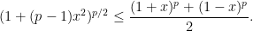
 ,
, 
![{r\in[0,1]}](https://s0.wp.com/latex.php?latex=%7Br%5Cin%5B0%2C1%5D%7D&bg=ffffff&fg=000000&s=0&c=20201002) , the numbers
, the numbers
![\displaystyle \forall A,B\in{\mathbb R},\quad \max_{r\in[0,1]}\{\alpha(r)|A|^p+\beta(r)B^p\}\le |A+B|^p+|A-B|^p.](https://s0.wp.com/latex.php?latex=%5Cdisplaystyle++%5Cforall+A%2CB%5Cin%7B%5Cmathbb+R%7D%2C%5Cquad+%5Cmax_%7Br%5Cin%5B0%2C1%5D%7D%5C%7B%5Calpha%28r%29%7CA%7C%5Ep%2B%5Cbeta%28r%29B%5Ep%5C%7D%5Cle+%7CA%2BB%7C%5Ep%2B%7CA-B%7C%5Ep.+&bg=ffffff&fg=000000&s=0&c=20201002)
 and
and  ; then it amounts to the monotonicity of a function).
 , set
, set  ,
,  ,
,  to get


 ,
,  . We show that
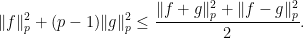
 and
and  (Ball-Carlen-Lieb). Heinavaara 2022 proves this for
  .
.
 .
.  such that for all
  ,
, 

 .
. , the set
  is orthogonal, so
 ,
, 
 . Then


 .
. , then

 , then

 has Rademacher cotype
  but no nontrivial martingale cotype.
 be an embedding of distorsion
  . Then

 .
. and
and  , as the least
  satisfying
![{[m]_p^n=(\{1,2,\ldots,n\},\|.\|_p)}](https://s0.wp.com/latex.php?latex=%7B%5Bm%5D_p%5En%3D%28%5C%7B1%2C2%2C%5Cldots%2Cn%5C%7D%2C%5C%7C.%5C%7C_p%29%7D&bg=ffffff&fg=000000&s=0&c=20201002) , viewed as an approximation of
, viewed as an approximation of  . What can one say about
 ![{c_q([m]_p^n)}](https://s0.wp.com/latex.php?latex=%7Bc_q%28%5Bm%5D_p%5En%29%7D&bg=ffffff&fg=000000&s=0&c=20201002) ?
? . Then


 .
. , the best we know now is
![\displaystyle \min\{n^{1/q - 1/p},m^{1- q/p}\}\le_{p,q}c_q([m]_p^n)\le_{p,q}\min\{n^{1/q - 1/p},m^{1- 2/p}\}.](https://s0.wp.com/latex.php?latex=%5Cdisplaystyle++%5Cmin%5C%7Bn%5E%7B1%2Fq+-+1%2Fp%7D%2Cm%5E%7B1-+q%2Fp%7D%5C%7D%5Cle_%7Bp%2Cq%7Dc_q%28%5Bm%5D_p%5En%29%5Cle_%7Bp%2Cq%7D%5Cmin%5C%7Bn%5E%7B1%2Fq+-+1%2Fp%7D%2Cm%5E%7B1-+2%2Fp%7D%5C%7D.+&bg=ffffff&fg=000000&s=0&c=20201002)
 and every
  , the metric space
  has a biLipschitz embedding into
  .
. .
.  , the space
 if for all
  , for all
  ,
, 
 , then the lefthand side is


 which has martingale type
 . But
. But
 has one sign changed. So
 has length


![\displaystyle c_q([m]_p^n)\ge c_q([2]_p^n)=c_q(\{-1,1\}^n,\|.\|_p).](https://s0.wp.com/latex.php?latex=%5Cdisplaystyle++c_q%28%5Bm%5D_p%5En%29%5Cge+c_q%28%5B2%5D_p%5En%29%3Dc_q%28%5C%7B-1%2C1%5C%7D%5En%2C%5C%7C.%5C%7C_p%29.+&bg=ffffff&fg=000000&s=0&c=20201002)
 (the other case is similar). Let
  have distorsion
 , and the lefthand side is bounded below by
  , so
, so  .
. with constant
  if for any
  such that any function
  satisfies
 .
. .
.  . Indeed, this would have many geometric applications.
 .
.  with
with ![{[m]_p^n}](https://s0.wp.com/latex.php?latex=%7B%5Bm%5D_p%5En%7D&bg=ffffff&fg=000000&s=0&c=20201002) . This is not a serious matter, since
. This is not a serious matter, since![\displaystyle [m]_p^n \subset {\mathbb Z}_{m}^{n}\subset [m+1]_p^{2n}.](https://s0.wp.com/latex.php?latex=%5Cdisplaystyle++%5Bm%5D_p%5En+%5Csubset+%7B%5Cmathbb+Z%7D_%7Bm%7D%5E%7Bn%7D%5Csubset+%5Bm%2B1%5D_p%5E%7B2n%7D.+&bg=ffffff&fg=000000&s=0&c=20201002)
![\displaystyle c_q([m]_p^n)\ge_{p,q} m^{1-\frac{q}{p}} \quad \text{ if }m\le n^{1/q},](https://s0.wp.com/latex.php?latex=%5Cdisplaystyle++c_q%28%5Bm%5D_p%5En%29%5Cge_%7Bp%2Cq%7D+m%5E%7B1-%5Cfrac%7Bq%7D%7Bp%7D%7D+%5Cquad+%5Ctext%7B+if+%7Dm%5Cle+n%5E%7B1%2Fq%7D%2C+&bg=ffffff&fg=000000&s=0&c=20201002)
![\displaystyle c_q([m]_p^n)\ge_{p,q} n^{\frac{1}{q}-\frac{1}{p}} \quad \text{ if }m\ge n^{1/q}.](https://s0.wp.com/latex.php?latex=%5Cdisplaystyle++c_q%28%5Bm%5D_p%5En%29%5Cge_%7Bp%2Cq%7D+n%5E%7B%5Cfrac%7B1%7D%7Bq%7D-%5Cfrac%7B1%7D%7Bp%7D%7D+%5Cquad+%5Ctext%7B+if+%7Dm%5Cge+n%5E%7B1%2Fq%7D.+&bg=ffffff&fg=000000&s=0&c=20201002)
 -distorsion, one can assume that
  have distorsion
  , whereas the right hand side is
  , so
, so  .
. , we define a martingale
 . We view
  as a smoothing operator.
 and
and  , let
, let  . Then


 , this what we want to see on the righthand side.
 with
with  mod
mod  . For fixed


 gives the expected bound
  .
.
 , over larger and larger boxes, of densities of packings in boxes.
 is denoted by
  , this is the sphere packing constant in
  . An
. An  .
. is an
is an  and the distance between two points (strings) is the number of coordinates where they differ.
 to your friend. You are provided with a device which converts such strings into strings of length
  from it. Thus he can correct the errors. Using his own converter, he can recover the original
  has been guessed for centuries: it is achieved by the hexagonal packing in the plane. The first published proof is due to the norwegian mathematician Axel Thue in 1910, but considered as insufficiently rigorous. In 1943, the hungarian mathematician Laszlo Fejes Toth published a complete proof. A good reference for this proof is Brass, Moser and Pach’s book on Research problems in discrete geometry. Other, simpler, proofs have been found since.
 requires a lot of 3-dimensional geometry, plus help from a computer.
 be a metric space. Let
  denote the set of values of
  is copositive if
 and all complex coefficients
  ,
, 

 . Suppose there exists a copositive function
  such that
  and
and 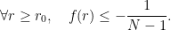
 -code in
 . q.e.d.
 over the field
  with
with  is a
is a  -dimensional subvectorspace of
  . It is an
  . This is optimal, as can be proved using a positive definite function on
  (which turns out to be a polynomial).
 is a
is a  -dimensional subvectorspace of
  . It is an
  .
. will be a Schwartz function, i.e. it is infinitely differentiable, and it decays, as well as all its derivatives, faster that any power of
  . To such a function
  , we associate the radial function
  on
on  .
. such that
  ,
,  .
. is nonnegative on
  .
. which is an
  is related to being positive definite.
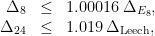
 and Leech denote very regular periodic configurations which exist only in those dimensions.
 that satisfies Cohn-Elkies’ assumptions in dimension
  . This implies that the
  .
.  that satisfies Cohn-Elkies’ assumptions in dimension
  for
for  . This implies that the Leech lattice has maximal density in
  .
.  is an algebraic group acting algebraically on an algebraic variety
  . Then
  acts on
  . We equip
  has
has  ,
,  triangular matrices,
  diagonal matrices,
  unipotent matrices. Then
  -orbits are the origin, two halflines and two halfplanes.
  is second countable and
  (topology separates points). This is known as Chevalley Theorem (combined with a result of Borel-Serre).
![{[0,1]}](https://s0.wp.com/latex.php?latex=%7B%5B0%2C1%5D%7D&bg=ffffff&fg=000000&s=0&c=20201002) .
.![{[0,1]\simeq\{ 0,1 \}^{\mathbb N}\simeq}](https://s0.wp.com/latex.php?latex=%7B%5B0%2C1%5D%5Csimeq%5C%7B+0%2C1+%5C%7D%5E%7B%5Cmathbb+N%7D%5Csimeq%7D&bg=ffffff&fg=000000&s=0&c=20201002) a separable Hilbert space.
a separable Hilbert space. ). Standard Borel sets have this property.
 ,
,  has a unique
  acting on projective space
  has no invariant measure in the Haar class. More generally, when
  is parabolic,
  has no invariant measure in the Haar class.
 is a closed normal subgroup, then
  has a finite invariant measure iff
 ![{V\rightarrow[0,1]}](https://s0.wp.com/latex.php?latex=%7BV%5Crightarrow%5B0%2C1%5D%7D&bg=ffffff&fg=000000&s=0&c=20201002) is a.e. constant. Here,
is a.e. constant. Here,  where
where  to an orbit. This must be a Borel and measure class isomorphism, thanks to the uniqueness of the Haar class.
![{[\nu]}](https://s0.wp.com/latex.php?latex=%7B%5B%5Cnu%5D%7D&bg=ffffff&fg=000000&s=0&c=20201002) on
on  in the class, there exists a family of
  on
on  , such that
  is a Haar measure on the orbit denoted by
![{[\bar{\nu}]}](https://s0.wp.com/latex.php?latex=%7B%5B%5Cbar%7B%5Cnu%7D%5D%7D&bg=ffffff&fg=000000&s=0&c=20201002) .
. is a normal
  has a finite Haar measure. By Noetherianity, there exists a minimal element
  among such cocompact normal
  ,
,  maps to a closed subset of
  hence is compact.
 ), then every
  acting on
  . It must be supported on a fixed point, i.e.
  . Then
  is a
is a 
 , for
, for  .
. has locally closed leaves.
 defined almost everywhere, up to almost everywhere equality. The space of such maps is denoted by
  .
. such that
  is a morphism.
 is ergodic.
 is ergodic.
 to a compact group
  , for every map
  (equipped with Haar measure),
  .
. .
. . Since probability measure is invariant,
  is equivariant and the action on
  is isometric. Now
  is a compact factor, one can assume
  . Take
  . The map
  is
is  , hence constant, so
  .
. . One can assume that metric space
  is compact. It must act transitively on
  . Under assumption 4,
  be a compact subgroup. Let
  be a homomorphism. Then the action of
  is not metrically ergodic.
 be a probability space. Then the shift action of
  is metrically ergodic.
 , and the shift action on
  is ergodic.
 be a lattice,
  a noncompact closed subgroup. Then the action of
  and the action of
  ). For the
 .
. is an amenable subgroup, the action of
  is amenable.
 .
. .
. and
and  is a
is a  such that
  .
.  . Every algebraic representation of this action is given by a pair
  and a point in
  in
in  to
to 
 , and for every AREA
  , we have a unique morphism
  such that
  .
. is an initial object in the category of AREAs of
 . This is nonempty. By Noetherianity, one can pick a minimal element
 . Composing with projection, we get a
  , hence an embedding
  up to conjugacy. By minimality,
  . The other projection
  provides us with a
  , which is unique.
 is unbounded (i.e. not contained in a compact subgroup). Then the initial object is trivial: any representation of
  . For
. For  the inclusion of
  .
.  which commutes with
  is a homothety.
 be a
be a  . Set
. Set
 is right-
 such that
  ,
,  , i.e.
  , by amenability, there exists an
  . Since
  is the stabilizer of a measure
  is constant, which contradicts the assumption that
  is a nontrivial AREA for
 ![{{\mathbb Z}[\sqrt{2}]}](https://s0.wp.com/latex.php?latex=%7B%7B%5Cmathbb+Z%7D%5B%5Csqrt%7B2%7D%5D%7D&bg=ffffff&fg=000000&s=0&c=20201002) is a lattice in
is a lattice in  .
.![{{\mathbb Z}[\frac{1}{p}]}](https://s0.wp.com/latex.php?latex=%7B%7B%5Cmathbb+Z%7D%5B%5Cfrac%7B1%7D%7Bp%7D%5D%7D&bg=ffffff&fg=000000&s=0&c=20201002) is a lattice in
is a lattice in  .
.![{SL_n({\mathbb Z}[\frac{1}{p}])}](https://s0.wp.com/latex.php?latex=%7BSL_n%28%7B%5Cmathbb+Z%7D%5B%5Cfrac%7B1%7D%7Bp%7D%5D%29%7D&bg=ffffff&fg=000000&s=0&c=20201002) is a lattice in
is a lattice in  .
. is irreducible if its projections to both factors are dense subgroups.
 and of
  on
on  are ergodic.
 on
on  is ergodic.
 equipped with the weak
 topology is continuous.
 . Any two are commensurable. Say a subgroup
  ,
,  and
and  be an irreducible lattice. Let
  be a compact open subgroup. Then
 . Hence
  is a lattice which is commensurated by the dense subgroup
  .
. where
where  is a lattice,
  is commensurated and
  is dense. Then one can reconstruct
  from these data. There exists a totally disconnected group
  , a dense embedding
  , and a precompact embedding
  such that
  is an irreducible lattice. It is called the Schlichting completion of
  .
. tdlc are simpler that lattices in Lie groups, in the sens that we have a dual way of looking at them.
 and
and  factors through one of the factors.
  , then
  .
.  which is amenable and metrically ergodic.
 is amenable and metrically ergodic.
 is nonempty, it is an
  ). Therefore, there exists an
  -map
-map  . I.e., there exists an
  . This proves amenability.
 is a.e. independant on the
  variable, and on the
  variable, therefore a.e. constant.
 is ergodic.
 is ergodic. Indeed, one can mod out by a proper action: the space of
  , denoted by
  , is well defined, since the diagonal
  .
.
 is implies by metric ergodicity of
  .
. . The ergodic action of
  ,
,  -map
-map  . By ergodicity, we get a map
  .
.
 . So the
  . There exists a gate
  where
where  . By ergodicity of the
  , where
  is the normalizer of
  ) from
  . Again by ergodicity, there is a
  ,
,  . So the above morphism to
  was to
  . The formula
 . In other words,
  . This implies that
  . Composing with the projection
  , we get
 , so
, so  . We have an
  (equivariant w.r.t.
  ).
). , the diagonal. This is an AREA of
  where
where  . Let us show that we are done if
  .
. .
.  is equal ti its own normalizer in
  , so
, so  ,
,  . It is amenable, noncompact, and its centralizer is the upper diagonal
  . The
. The  acts on
  .
. -buildings, covered by Caprace-Lecureux. At infinity, such buildings have an exotic projective plane. It has a large group of projectivities (in fact a pseudogroup of maps from lines to lines). This yields a large group acting on the boundary of a tree. It plays the role of
  . It is not too hard to show that this group is linear iff the building is classical. It follows that
  yet.
yet. that commutes with
  ,
, which is
  -equivariant.
 be a lattice. Assume that the action of
  is ME. Then there exists an initial object (a gate), i.e. a
  -equivariant map
 and
and  .
.  . By amenability and ME, there exists a proper subgroup
  , under homomorphism
  . The gate will be a deeper object, but this suffices to prove that the gate is nontrivial.
 -actions, i.e.
 into the right action of
  on
on  .
. on
on  . To a morphism
  given by element
  of algebraic varieties
  .
. . The group
  . On the other hand,
  . This homomorphism
  .
. normalize each other. Then they have the same gate
  generating
  commutes with
  .
. . The first three
  , equivariant with respect to
  . By ergodicity, the
  , i.e; b y
  .
. , equivariant with respect to
  .
.![{k[G]}](https://s0.wp.com/latex.php?latex=%7Bk%5BG%5D%7D&bg=ffffff&fg=000000&s=0&c=20201002) , to
, to  . It is injective, since its Zariski support is
  . The gate
  ,
,  ,
,  ,
,  ,… denote the
  be a parabolic. If
  , then
  ,
,  hence
hence  ,
,  .
. generate
  and a
and a  , equivariant with respect to
  .
.  is noncompact. By a finite number of up and down steps of taking normalizers we reach
  . Then the
  -gate equals the
  , contradiction.
 and
and  .
.  where
where  . Le
. Le  such that
  up to conjugation and finite index.
 . I.e. for every embedding
  to a local field, either
  is precompact or
  and
and  .
.  . Can assume that it is adjoint. For every embedding
  is precompact unless
  infinitely many immersed maximal totally geodesic subspaces of dimension
  , then the assumption of Lemma 24 holds for all
  ,
,  , the group
  is compatible. In particular, if there exist infinitely many immersed maximal totally geodesic subspaces of dimension
  ).
). be a map. The Greg is the data
  .
.  ,
,  ,
,  ,
,  shift,
  projection to the
  , a probability measure on the set of edges emanating from
  set of paths in the graph,
  some Gibbs measure associate. Decorate edges with elements of
  .
. denote the unit tangent bundle of
  geodesic flow. Let
  . Fix a fundamental domain. For each time
  which tells which group element drags
  back to the fundamental domain. One can decorate the picture with a flat bundle.
 , let
, let  . Assume that
  .
. equipped with the future
  . Let
. Let  equipped with the past
  (I view these as factors of
  ,
,  . It turns out that
  , using the natural extension construction.
 be a pmp map which is not invertible. One constructs another system, with an invertible transformation, by taking the inverse limit
  of
of
 ,
,  .
. on
on  (i.e. a family of complete separable metric spaces on which a lift of
  ,
,  , and for
  ,
,

 is defined by
 on
on  and
and  , when modded out by
  and
and  . If instead one mods out by
  , one gets the space
  of
of  and
and  . I think of these as ideal futures and pasts.
 and
and  are amenable
  is measure class preserving.
  is called a Boundary pair. The spaces are amenable and the maps
  and
and  and measurable equivariant maps
  ,
,  and
and  .
. is the minimal parabolic.
  -valued metric on
  be the composition of
  with
with 
 converges to an interior point of the Weyl chamber
 of a graph
  be the number of independent sets of size
 . Subdivision is allowed. How many faces are needed? Let
  be the number of faces of dimension
 . For a
  , the numbers of triangles and edges must satisfy
 and
and  . The point is that the modification changed only the left-hand side of the inequality.
 .
. be any infinite field. Let
  be the ideal generated by all monomials which are not supported on
 ![\displaystyle \mathbf{k}[\Delta]=\mathbf{k}[X]/I_\Delta.](https://s0.wp.com/latex.php?latex=%5Cdisplaystyle+%5Cmathbf%7Bk%7D%5B%5CDelta%5D%3D%5Cmathbf%7Bk%7D%5BX%5D%2FI_%5CDelta.+&bg=ffffff&fg=000000&s=0&c=20201002)
![\displaystyle H(\mathbf{k}[\Delta],t)=\frac{1}{(1-t)^d }\sum f_{i-1}(\Delta)t^i(1-t)^{d-i}.](https://s0.wp.com/latex.php?latex=%5Cdisplaystyle+H%28%5Cmathbf%7Bk%7D%5B%5CDelta%5D%2Ct%29%3D%5Cfrac%7B1%7D%7B%281-t%29%5Ed+%7D%5Csum+f_%7Bi-1%7D%28%5CDelta%29t%5Ei%281-t%29%5E%7Bd-i%7D.+&bg=ffffff&fg=000000&s=0&c=20201002)
 ,
,![\displaystyle H(\mathbf{k}[\Delta],t)=\sum_{k,i}{k\choose i}f_{i-1}(\Delta)t^k.](https://s0.wp.com/latex.php?latex=%5Cdisplaystyle+H%28%5Cmathbf%7Bk%7D%5B%5CDelta%5D%2Ct%29%3D%5Csum_%7Bk%2Ci%7D%7Bk%5Cchoose+i%7Df_%7Bi-1%7D%28%5CDelta%29t%5Ek.+&bg=ffffff&fg=000000&s=0&c=20201002)
![{\mathbf{k}[\Delta]}](https://s0.wp.com/latex.php?latex=%7B%5Cmathbf%7Bk%7D%5B%5CDelta%5D%7D&bg=ffffff&fg=000000&s=0&c=20201002) , we pick a matrix
, we pick a matrix  whose rows are linear combinations of vertices. The quotient
![\displaystyle A(\Delta,\Theta)=\mathbf{k}[\Delta]/<\Theta>](https://s0.wp.com/latex.php?latex=%5Cdisplaystyle+A%28%5CDelta%2C%5CTheta%29%3D%5Cmathbf%7Bk%7D%5B%5CDelta%5D%2F%3C%5CTheta%3E+&bg=ffffff&fg=000000&s=0&c=20201002)
 . This holds generically.
![\displaystyle H(\mathbf{k}[\Delta],t)=\frac{1}{(1-t)^d }h(t),](https://s0.wp.com/latex.php?latex=%5Cdisplaystyle+H%28%5Cmathbf%7Bk%7D%5B%5CDelta%5D%2Ct%29%3D%5Cfrac%7B1%7D%7B%281-t%29%5Ed+%7Dh%28t%29%2C+&bg=ffffff&fg=000000&s=0&c=20201002)

 can be computed as follows. Write a Pascal triangle with
  .
. as a fan. Consider the algebra
  of cone-wise polynomial functions. If
  of
of  , where
  is
is  , the pairing
 is perfect.
 or
or  (induced by other
  is shellable of codimension
 , where
  is the minimal simplex of
  (everything here once modded out by
  , I first express it in shelling steps. The shelling turned around (in reverse order), is a shelling too. Therefore I can construct an element
  is expressible in terms of cone-wise polynomials:
 be a cone-wise linear function. Assume that
  , multiplication with
  yields an isomorphism
  .
. , is an M-vector (i.e. realizable as the dimensions in a polynomial ring). Define, for
  ,
,
 as follows.
 is the kernel of the multiplication by

 is definite of sign
  on
on  be two strictly convex elements of
  . The restriction of
  to the span of

 satisfies
 -sphere
  . Faces provide a generating system for
  (because
 , which is larger than the Krull dimension of
  . Later on we shall see a model for
  -faces, therefore
 . Indeed, by Poincaré duality and if Lefschetz property applies to

 of
of  for all nonzero
  .
. , the map to stars of vertices


![\displaystyle 0\rightarrow \mathbf{k}[st_v\Sigma]\rightarrow \mathbf{k}[\Sigma]\rightarrow\mathbf{k}[\Sigma - v]\rightarrow 0](https://s0.wp.com/latex.php?latex=%5Cdisplaystyle+0%5Crightarrow+%5Cmathbf%7Bk%7D%5Bst_v%5CSigma%5D%5Crightarrow+%5Cmathbf%7Bk%7D%5B%5CSigma%5D%5Crightarrow%5Cmathbf%7Bk%7D%5B%5CSigma+-+v%5D%5Crightarrow+0+&bg=ffffff&fg=000000&s=0&c=20201002)


 . The tensor product
 is isomorphic to the cohomology
 is not Poincaré duality, but the quotient
 . The kernel is always
  . Then $latex {B^(\mu)}&fg=000000$ is a minimal quotient of $latex {A^(\Delta)}&fg=000000$ such that
  is isomorphic to
  be an element in
  which is dual to
 is the minor of
  (and generic
  satisfies the Hard Lefschetz theorem.
 be a strictly convex cone-wise linear function.
 is an isomorphism.
  is definite of sign
  .
. -sphere. Thee exists
  such that
 ,
,  , consider the monomial ideal generated by
  in
in  such that
  . For every vertex
  . The restriction of
  is nonzero. Since

 . The sum is strictly positive. This proves that
  , and HL follows.
 is the boundary of the
 ![{A(\Sigma_0)={\mathbb R}[x]/x^{d+1}}](https://s0.wp.com/latex.php?latex=%7BA%28%5CSigma_0%29%3D%7B%5Cmathbb+R%7D%5Bx%5D%2Fx%5E%7Bd%2B1%7D%7D&bg=ffffff&fg=000000&s=0&c=20201002) , and HR is proven by direct calculation.
, and HR is proven by direct calculation. . What we observe are Pachner moves: – flip of diagonals in a quadrilateral face, – upraisal of a vertex in the middle of a face. In the first case, there is a common refinement (blow up by adding a vertex at the intersection of diagonals). I denote by
  ). I call
  the side where this minimal cardinality is smallest. I denote by
  the flip locus after the flip (it is the star of the minimal simplex introduced). Then
 .
. is the ring of cone-wise polynomials on
 ![\displaystyle \mathbf{k}[A,B]=I_B/I_A,](https://s0.wp.com/latex.php?latex=%5Cdisplaystyle+%5Cmathbf%7Bk%7D%5BA%2CB%5D%3DI_B%2FI_A%2C+&bg=ffffff&fg=000000&s=0&c=20201002)
 is the ideal generated by monomials whose support is not in

 is in homogeneity degree
  is in homogeneity degree
  . Thus, for
  , the maps
 , the maps
 truncated after
  . This decomposition is orthogonal with respect to the Poincaré pairing. Indeed, if
  has degree
  and
and  has degree
  , then
  which injects into
  , therefore
  . If instead
  of minimal face
 .
. where
where  (ordered by inclusion) is a set of subsets of
  ,
,  .
. .
. , the set
  partitions
  .
. associated to
  , is defined as follows. Let $latex {(e_i)_{i\in E}}&fg=000000$ be a generating set in
  . For every subset
  , set $latex {e_F=\sum_{i\in F} e_i}&fg=000000$. To a flag
  of
of  . Then the fan
  . The fan consists of 6 cones in the plane.
 ). Hard Lefschetz. Hodge-Riemann.
 satisfies
 , a matroid can be reduced in two ways:
 .
. .
. )
)

 ?
? alternate in signs and their absolute values are unimodal, i.e. increase and then decrease.


 , and
, and
![{[\alpha_j]\in A(B _n)}](https://s0.wp.com/latex.php?latex=%7B%5B%5Calpha_j%5D%5Cin+A%28B+_n%29%7D&bg=ffffff&fg=000000&s=0&c=20201002) (resp. all
(resp. all ![{[\beta_j]}](https://s0.wp.com/latex.php?latex=%7B%5B%5Cbeta_j%5D%7D&bg=ffffff&fg=000000&s=0&c=20201002) ) are the same (independent of
) are the same (independent of  ). This is because one mods out by global linear functions. Denote them by
  is a coefficient; merely explain its combinatorial content.
 matrix which is indefinite, so the determinant is negative.
 does not degenerate on squarefree monomial ideals.
 . The first nontrivial isomorphism is multiplication by
  .
. is restriction to the star of
  . Its image is
  . Let
. Let  be an other vertex. One expects that the kernel of multiplication with a generic linear combination of
  be as small as possible, i.e.
  . Dually, the image of this combination should be
  . Now
. Now  be linear maps such that
  and
and  intersect trivially. Then the kernel of a generic linear combination of
  .
. and
and  .
. and
and  is the orthogonal complement of
  .
. , the kernel of the multiplication is the intersection of kernels. If we can do it for
  all vertices, we shall be done for Hard Lefschetz.
 .
.  , hence we continue the linear forms with
 . Then
  .
.
 the two hemispheres determined by
 .
.

 of
of  in degree
  in degree
  , the annihilator of
  , hence

 . Before Artinian reduction, the map
![\displaystyle 0\rightarrow \mathbf{k}[D,\partial D]\rightarrow \mathbf{k}[D]\rightarrow\mathbf{k}[\partial D]\rightarrow 0](https://s0.wp.com/latex.php?latex=%5Cdisplaystyle+0%5Crightarrow+%5Cmathbf%7Bk%7D%5BD%2C%5Cpartial+D%5D%5Crightarrow+%5Cmathbf%7Bk%7D%5BD%5D%5Crightarrow%5Cmathbf%7Bk%7D%5B%5Cpartial+D%5D%5Crightarrow+0+&bg=ffffff&fg=000000&s=0&c=20201002)
 is a regular system of parameters for
  , and the sequence remains exact when modding out by
  -sphere, by Poincaré duality, multiplication by
 ![\displaystyle \mathbf{k-1}[\partial D]/\tilde\Theta \rightarrow \mathbf{k}[\partial D]/\tilde\Theta](https://s0.wp.com/latex.php?latex=%5Cdisplaystyle+%5Cmathbf%7Bk-1%7D%5B%5Cpartial+D%5D%2F%5Ctilde%5CTheta+%5Crightarrow+%5Cmathbf%7Bk%7D%5B%5Cpartial+D%5D%2F%5Ctilde%5CTheta+&bg=ffffff&fg=000000&s=0&c=20201002)
 is a lower dimension sphere, this allows for induction.
 where
where  -acyclic over
  is a trivial case.
 .
.
 satisfies bpp if and only if the composition
 is an isomorphism.

 satisfies bpp in general?
 . The idea is to construct a hypersurface
  is isomorphic to
  .
. , the subdivision, and there is an orthogonal decomposition
 consists of all monomials not in
 of
of 
 is not exactly the hypersurface we need. Every element of the kernel of that map can be killed by introducing holes. This produces a hypersurface with boundary
  , a closed hypersurface, in a new
  which is still a homology sphere. By diagram chasing, one shows that
  satisfies bpp if and only if
  does,
does,
 covers the general case.

 . Then Hard Lefschetz holds for
  satisfies bpp in degree
  satisfies bpp. We manage to find a refinement
  where
where  is a simplicial complex and
  .
.![\displaystyle A(|\mu|,\Theta)=\mathbf{k}[X]/I(\mu).](https://s0.wp.com/latex.php?latex=%5Cdisplaystyle+A%28%7C%5Cmu%7C%2C%5CTheta%29%3D%5Cmathbf%7Bk%7D%5BX%5D%2FI%28%5Cmu%29.+&bg=ffffff&fg=000000&s=0&c=20201002)
 , hence of
  . Let
. Let  be the smallest quotient of
  such that
  . Then
 , then
  for all nonzero elements
  .
.

 satisfies Hard Lefschetz.
 as follows. For
  , set
, set
 denotes the minor in the matrix
  , then
  . Then
 . We want to establish this by only considering
  .
.![{[-1,1]\times\mu/\sim}](https://s0.wp.com/latex.php?latex=%7B%5B-1%2C1%5D%5Ctimes%5Cmu%2F%5Csim%7D&bg=ffffff&fg=000000&s=0&c=20201002) where
where  and
and  are collapsed to distinct points
  is a
is a  . Projection along
  for
for  . The following are equivalent:
 in
in  in degree
  .
. be a subcomplex. If
 is the quotient of
  obtained like
 of
of  at the level of the suspension. Restricting to
  is generated by squarefree monomials in each graded component.
![{\mathbf{k}[K]}](https://s0.wp.com/latex.php?latex=%7B%5Cmathbf%7Bk%7D%5BK%5D%7D&bg=ffffff&fg=000000&s=0&c=20201002) . Since
. Since  where
where ![\displaystyle \mathrm{deg}(x_\tau^2)=\sum_{F\text{ facet of }|\mu|\text{ containing }\tau}\mathrm{deg}(x_F)\frac{\prod_{i\subset\tau}[\Theta_{F\setminus i}]}{\prod_{j\in F\setminus\tau}[\Theta_{F\setminus j}]}.](https://s0.wp.com/latex.php?latex=%5Cdisplaystyle+%5Cmathrm%7Bdeg%7D%28x_%5Ctau%5E2%29%3D%5Csum_%7BF%5Ctext%7B+facet+of+%7D%7C%5Cmu%7C%5Ctext%7B+containing+%7D%5Ctau%7D%5Cmathrm%7Bdeg%7D%28x_F%29%5Cfrac%7B%5Cprod_%7Bi%5Csubset%5Ctau%7D%5B%5CTheta_%7BF%5Csetminus+i%7D%5D%7D%7B%5Cprod_%7Bj%5Cin+F%5Csetminus%5Ctau%7D%5B%5CTheta_%7BF%5Csetminus+j%7D%5D%7D.+&bg=ffffff&fg=000000&s=0&c=20201002)
 for
for  denote the element used to define the degree. Then
  is
is
 In particular, in characteristic
 , then
  is independent of
  .
. . By Poincare duality, because
  . The ideal of
  , and
, and  is again a cycle.
  is generated by
  ,
, 


 .
. of
of  is a single face
  .
. is any other face in
  is a simplex
  , face of
  is independent of one of the variables of
  .
. using a second copy of
  obtained by replacing
  with
with  .
.
 , one gets
 . If
. If  , then so are
  and
and  .
. for some subcomplex
  if
if  , hence
  .
. has dimension
  is represented by an element
  such that the support of
  . Furthermore,
  is generated by a single element in top degree. This combines into compatibility.
 ,
,  is Cohen-Macaulay.
 , there exists
  such that
  (see Stanley’s book).
 . Let us define
 . Thus we get
 are increasing while
  a sequence of finite index subgroups. Let
 ![\displaystyle \lim_{i\rightarrow\infty}\frac{b_k(\Gamma_i,F)}{[\Gamma:\Gamma_i]}](https://s0.wp.com/latex.php?latex=%5Cdisplaystyle++%5Clim_%7Bi%5Crightarrow%5Cinfty%7D%5Cfrac%7Bb_k%28%5CGamma_i%2CF%29%7D%7B%5B%5CGamma%3A%5CGamma_i%5D%7D+&bg=ffffff&fg=000000&s=0&c=20201002)
 , i.e. acts freely on a
  grows at most like the number of cells of
  , i.e. linearly with the index. Also, the Euler characteristic is proportional to the index, therefore linear growth is to be expected.
 and
and  are nested normal subgroups, then the limit exists and for all
  ,
, ![\displaystyle \lim_{i\rightarrow\infty}\frac{b_j(\Gamma_i,{\mathbb R})}{[\Gamma:\Gamma_i]}=b_j^{(2)}(\Gamma)](https://s0.wp.com/latex.php?latex=%5Cdisplaystyle++%5Clim_%7Bi%5Crightarrow%5Cinfty%7D%5Cfrac%7Bb_j%28%5CGamma_i%2C%7B%5Cmathbb+R%7D%29%7D%7B%5B%5CGamma%3A%5CGamma_i%5D%7D%3Db_j%5E%7B%282%29%7D%28%5CGamma%29+&bg=ffffff&fg=000000&s=0&c=20201002)
 -Betti number.
  has nonpositively curved left-invariant metrics, hence is contractible. Lattices exist, thery need not be cocompact. Nevertheless, they have finite covolume
  .
. , the relative volume of the
  -thin part tends to zero.
  .
.
 of
of  , and all
  ,
, ![\displaystyle \lim_{i\rightarrow\infty}\log|H_k(\Gamma(N),{\mathbb Z})_{tor}|=o([\Gamma:\Gamma(N)]^{n/(n+1)}).](https://s0.wp.com/latex.php?latex=%5Cdisplaystyle++%5Clim_%7Bi%5Crightarrow%5Cinfty%7D%5Clog%7CH_k%28%5CGamma%28N%29%2C%7B%5Cmathbb+Z%7D%29_%7Btor%7D%7C%3Do%28%5B%5CGamma%3A%5CGamma%28N%29%5D%5E%7Bn%2F%28n%2B1%29%7D%29.+&bg=ffffff&fg=000000&s=0&c=20201002)
 is
is ![{|Y_i|=o([\Gamma:\Gamma_i])}](https://s0.wp.com/latex.php?latex=%7B%7CY_i%7C%3Do%28%5B%5CGamma%3A%5CGamma_i%5D%29%7D&bg=ffffff&fg=000000&s=0&c=20201002) .
.
 is finite.
 is of class
  .
.
 for every normal chain
  .
.  . Using standard homotopy theory (see Geoghegan’s book, the keyword in stack of CW complexes), one glues together spaces
  into a space
  with fibers
  .
.
![\displaystyle [\Gamma_\sigma\cap\Gamma_i]=\sum_{\sigma\in \Gamma_i\setminus\Delta}[\Gamma:\Gamma_{\sigma,i}]](https://s0.wp.com/latex.php?latex=%5Cdisplaystyle++%5B%5CGamma_%5Csigma%5Ccap%5CGamma_i%5D%3D%5Csum_%7B%5Csigma%5Cin+%5CGamma_i%5Csetminus%5CDelta%7D%5B%5CGamma%3A%5CGamma_%7B%5Csigma%2Ci%7D%5D+&bg=ffffff&fg=000000&s=0&c=20201002)
![\displaystyle |Y_{\sigma,i}|=o(\frac{[\Gamma:\Gamma_{\sigma,i}]}{[{\mathbb Z}^{n_\sigma}:{\mathbb Z}^{n_\sigma}\cap\Gamma_{i}]}).](https://s0.wp.com/latex.php?latex=%5Cdisplaystyle++%7CY_%7B%5Csigma%2Ci%7D%7C%3Do%28%5Cfrac%7B%5B%5CGamma%3A%5CGamma_%7B%5Csigma%2Ci%7D%5D%7D%7B%5B%7B%5Cmathbb+Z%7D%5E%7Bn_%5Csigma%7D%3A%7B%5Cmathbb+Z%7D%5E%7Bn_%5Csigma%7D%5Ccap%5CGamma_%7Bi%7D%5D%7D%29.+&bg=ffffff&fg=000000&s=0&c=20201002)
![{|Y_i|=o([\Gamma:\Gamma_{\sigma,i}])}](https://s0.wp.com/latex.php?latex=%7B%7CY_i%7C%3Do%28%5B%5CGamma%3A%5CGamma_%7B%5Csigma%2Ci%7D%5D%29%7D&bg=ffffff&fg=000000&s=0&c=20201002) and proves a weak form of Theorem 4. To win an exponent, we need control on norms of differentials.
and proves a weak form of Theorem 4. To win an exponent, we need control on norms of differentials. -parabolics, and cells are incidents when parabolics are contained in each other. Vertices are maximal parabolics et top dimensional celles correspond to Borel subgroups. This complex is homotopic to a wedge of
  -spheres. The cell stabilizers are intersections of
  ).
). . We want to estimate
  , assuming that injectivity radius tends to infinity.
 . Start with any representative, typically of length
  . If two pieces of the cycle are nearby, I can remove these pieces. Mod
  be finitely generated subgroups of a free group


 in a product of groups which are either Lie or tree automorphism groups. Example:
 ![{SL_2({\mathbb Z}[\sqrt{2}])<SL_2({\mathbb R})^2}](https://s0.wp.com/latex.php?latex=%7BSL_2%28%7B%5Cmathbb+Z%7D%5B%5Csqrt%7B2%7D%5D%29%3CSL_2%28%7B%5Cmathbb+R%7D%29%5E2%7D&bg=ffffff&fg=000000&s=0&c=20201002) .
.  in a surface
  of length
  is
is  , where
  are known.
 s,
s,  ,…
,… is
is  -Anosov if for every element
  ,
, 
 are singular values.
![\displaystyle P_W(q)=\sum_{u\in [e,w]}q^{\ell(u)}](https://s0.wp.com/latex.php?latex=%5Cdisplaystyle++P_W%28q%29%3D%5Csum_%7Bu%5Cin+%5Be%2Cw%5D%7Dq%5E%7B%5Cell%28u%29%7D+&bg=ffffff&fg=000000&s=0&c=20201002)
 being palindromic. There is a criterion for that.
 -approximation of a Cayley graph
  is a finite graph
  and
and  form a completion of the semigroup of positive linear combinations of quasiconvex subgroups. Reduced rank gives rise to a morphism to
 .
. . Such groups also slightly a slightly weakened form of property (*).
 ,
,  ,
,  , for instance.
 cube complex without global fixed point, for any generating set, either
  that generate a free subgroup. This applies to Higman’s group (which acts of a
  ).
). be elements such that
 ![{\gamma=\prod[\gamma_i,\gamma_j]}](https://s0.wp.com/latex.php?latex=%7B%5Cgamma%3D%5Cprod%5B%5Cgamma_i%2C%5Cgamma_j%5D%7D&bg=ffffff&fg=000000&s=0&c=20201002) commutes with the others. Then in any finite dimensional unitary representation of
commutes with the others. Then in any finite dimensional unitary representation of  for every
  , when is the subgroup
  they generate free?
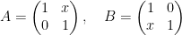
 , where it is easier, because ping-pong is easier there.
 generate
  is not, since the first Betti number of a Kähler manifold is always even (Hodge theory).
 . The outer automorphism group
  ,
,  . One picks a sequence
  and let act successively
  . One orbit in
  on the boundary. The temperature satisfies
 functions on
  .
. is
is  ,
, 
 denotes the space of bounded harmonic functions.
  , there exists a standard probability
  such that
 . Morally,
  the hitting measure. This is litterally true when
  is one point and
  has only constant functions in it.
  mass on
 is the set of nonamenable groups.
  , there exists
  such that
  .
. 